Demo 2: Differentiability

Demo by Christian Mikkelstrup, Hans Henrik Hermansen, Karl Johan Måstrup Kristensen and Magnus Troen. Revised March 2026 by shsp.

from sympy import *
from dtumathtools import *
init_printing()

When it comes to Python/CAS and differentiability, we face the same difficulties as with continuity. Python/CAS is not very suitable for proving differentiability. It is, however, a powerful tool once differentiability is established. In this demo we will show how Python can be of great use in work with differentiable functions.

Defining and Evaluating Vector Functions

Vector functions of multiple variables as defined in the textbook can be written as

\[\begin{split}\boldsymbol{f}(\boldsymbol{x}) = \begin{bmatrix} f_1(\boldsymbol{x}) \\ \vdots \\ f_k(\boldsymbol{x}) \end{bmatrix},\end{split}\]

where the coordinate functions \(f_1,\ldots,f_k\) in the output are scalar functions.

In Sympy, vector functions can be constructed using the Matrix object:

x1, x2, x3 = symbols('x1:4')

f_expr = Matrix([
    x1 * sin(x2) + x3**2,
    x1*x2*x3,
    x1**2 + 4*x2 * x3
])
f_expr

\[\begin{split}\displaystyle \left[\begin{matrix}x_{1} \sin{\left(x_{2} \right)} + x_{3}^{2}\\x_{1} x_{2} x_{3}\\x_{1}^{2} + 4 x_{2} x_{3}\end{matrix}\right]\end{split}\]

We can evaluate this vector function for a chosen input using .subs():

f_expr.subs({x1: 1, x2: 2, x3: 3})

\[\begin{split}\displaystyle \left[\begin{matrix}\sin{\left(2 \right)} + 9\\6\\25\end{matrix}\right]\end{split}\]

Note that this actully just shows that .subs() carries out the substitution on every entry in vector. If you prefer defining mathematical functions as Python functions, the same can be achieved with

def f(x1, x2, x3):
    return Matrix([
        x1 * sin(x2) + x3**2,
        x1*x2*x3,
        x1**2 + 4 * x2 * x3
    ])

f(x1,x2,x3)

\[\begin{split}\displaystyle \left[\begin{matrix}x_{1} \sin{\left(x_{2} \right)} + x_{3}^{2}\\x_{1} x_{2} x_{3}\\x_{1}^{2} + 4 x_{2} x_{3}\end{matrix}\right]\end{split}\]

f(1,2,3)

\[\begin{split}\displaystyle \left[\begin{matrix}\sin{\left(2 \right)} + 9\\6\\25\end{matrix}\right]\end{split}\]

Both approaches yield the same result. Which method you choose is up to personal preference.

The Gradient Vector

An example of a vector function is the gradient of a scalar function \(f:\Bbb R^n\to\Bbb R\):

\[\nabla f(\boldsymbol{x})=\left(\frac{\partial f}{\partial x_1}(\boldsymbol{x}),\frac{\partial f}{\partial x_2}(\boldsymbol{x}),\ldots, \frac{\partial f}{\partial x_n}(\boldsymbol{x})\right).\]

This can be considered as a map \(\nabla f: \mathbb R^n \to \mathbb R^n\). In demo 1 we showed how the gradient of a scalar function can be interpreted and visualized as a vector field. This is possible precisely because the number of coordinate functions in the output equals the number of input variables, e.g. both being \(\Bbb R^n\).

As an example we will consider the gradient of the function \(f: \mathbb{R}^2 \to \mathbb{R}\), defined by \(f(\boldsymbol{x}) = 1 - \frac{x_1^2}{2} -\frac{x_2^2}{2}\):

x1, x2 = symbols('x1:3')
f = 1 - x1**2 / 2 - x2**2 / 2

Nabla = dtutools.gradient(f)

f, Nabla

\[\begin{split}\displaystyle \left( - \frac{x_{1}^{2}}{2} - \frac{x_{2}^{2}}{2} + 1, \ \left[\begin{matrix}- x_{1}\\- x_{2}\end{matrix}\right]\right)\end{split}\]

We here see that the gradient \(\nabla f: \mathbb R^2 \to \mathbb R^2\) is given by \(\nabla f(x_1, x_2) = (-x_1, -x_2)\). Evaluating at a point, such as \(\boldsymbol{x}_0 = (1, -1)\), means computing the specific gradient vector associated with that point:

Nabla.subs({x1: 1, x2: -1})

\[\begin{split}\displaystyle \left[\begin{matrix}-1\\1\end{matrix}\right]\end{split}\]

Directional Derivatives

Consider again the function \(f: \mathbb{R}^2 \to \mathbb{R}\) with the functional expression \(f(\boldsymbol{x}) = 1 - \frac{x_1^2}{2} -\frac{x_2^2}{2}\).

We wish to find the directional derivative of \(f\) at the point \(\boldsymbol{x_0} = (1,-1)\), meaning the slope at this point on the graph, in the direction given by the direction vector \(\boldsymbol{v}=(-1,-2)\).

x0 = Matrix([1,-1])
v = Matrix([-1,-2])
x0, v

\[\begin{split}\displaystyle \left( \left[\begin{matrix}1\\-1\end{matrix}\right], \ \left[\begin{matrix}-1\\-2\end{matrix}\right]\right)\end{split}\]

The textbooks provides the following formula for the directional derivative that uses an inner product:

\[\nabla_{\boldsymbol{e}} f(\boldsymbol{x_0}) = \braket{\boldsymbol{e},\nabla f(\boldsymbol{x_0})},\]

where \(\boldsymbol e\) represents a unit direction vector, meaning a direction vector with a magnitude of \(1\). So, let us firstly normalize \(\boldsymbol v\), e.g. using the command .normalize() (alternatively, find and then divide by the norm):

e = v.normalized()
e

\[\begin{split}\displaystyle \left[\begin{matrix}- \frac{\sqrt{5}}{5}\\- \frac{2 \sqrt{5}}{5}\end{matrix}\right]\end{split}\]

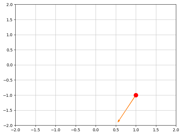
Let’s make a quick plot to see the point and the direction in the domain:

p1 = dtuplot.scatter(x0, rendering_kw={"markersize":10,"color":'r'}, xlim=[-2,2],ylim=[-2,2],show=False)
p1.extend(dtuplot.quiver(x0,e,show=False))
p1.show()

Next, we need the gradient of \(f\) at \(\boldsymbol{x_0}\):

Nabla = Matrix([diff(f,x1),diff(f,x2)]).subs({x1:x0[0],x2:x0[1]})
Nabla

\[\begin{split}\displaystyle \left[\begin{matrix}-1\\1\end{matrix}\right]\end{split}\]

We now have all necessary components. As we are dealing with real vectors (from \(\Bbb R^n\)), the inner product is calculated as the usual dot product, \(\nabla_{\boldsymbol{e}} f(\boldsymbol{x_0}) = \braket{\boldsymbol{e},\nabla f(\boldsymbol{x_0})}=\boldsymbol{e}\cdot \nabla f(\boldsymbol{x_0})\):

e.dot(Nabla)

The Hessian Matrix

The second-order partial derivatives of scalar functions will turn out to be important later in the course (for extremum characterization and Taylor approximation). The textbook conveniently gathers all 2nd-order partial derivatives into a matrix known as the Hessian matrix.

Let’s consider the following scalar function of three variables:

f = 1-x1**2/2-x2**3/2*x3 + x1*x3
f

Its Hessian matrix can be constructed manually as follows:

fx1x1 = f.diff(x1,2)
fx1x2 = f.diff(x1,x2)
fx1x3 = f.diff(x1,x3)
fx2x2 = f.diff(x2,2)
fx2x3 = f.diff(x2,x3)
fx3x3 = f.diff(x3,2)

H1 = Matrix([
    [fx1x1, fx1x2, fx1x3],
    [fx1x2, fx2x2, fx2x3],
    [fx1x3, fx2x3, fx3x3]
])

H1

\[\begin{split}\displaystyle \left[\begin{matrix}-1 & 0 & 1\\0 & - 3 x_{2} x_{3} & - \frac{3 x_{2}^{2}}{2}\\1 & - \frac{3 x_{2}^{2}}{2} & 0\end{matrix}\right]\end{split}\]

Or we can more conveniently use the .hessian command from the dtutools package:

H2 = dtutools.hessian(f)
H2

\[\begin{split}\displaystyle \left[\begin{matrix}-1 & 0 & 1\\0 & - 3 x_{2} x_{3} & - \frac{3 x_{2}^{2}}{2}\\1 & - \frac{3 x_{2}^{2}}{2} & 0\end{matrix}\right]\end{split}\]

Either way, we can evaluate the Hessian matrix at a chosen point with .subs():

H1.subs({x1:1,x2:2,x3:3}), H2.subs({x1:1,x2:2,x3:3})

\[\begin{split}\displaystyle \left( \left[\begin{matrix}-1 & 0 & 1\\0 & -18 & -6\\1 & -6 & 0\end{matrix}\right], \ \left[\begin{matrix}-1 & 0 & 1\\0 & -18 & -6\\1 & -6 & 0\end{matrix}\right]\right)\end{split}\]

The Jacobian Matrix

As the coordinate functions of a vector function themselves are scalar functions, then each coordinate function has a gradient. The textbook merges these gradients as rows in a new matrix known as the Jacobian matrix of the vector function:

\[\begin{split} \boldsymbol{J_f} = \begin{bmatrix} \nabla f_1^T\\ \nabla f_2^T \\ \nabla f_3^T\end{bmatrix}. \end{split}\]

For an example, consider the vector function \(\boldsymbol{f}: \mathbb{R}^4 \to \mathbb{R}^3\) defined by:

\[\begin{split} \boldsymbol{f} (\boldsymbol{x}) = \begin{bmatrix} f_1(\boldsymbol{x})\\ f_2(\boldsymbol{x})\\ f_3(\boldsymbol{x}) \end{bmatrix} = \left[\begin{matrix}x_{1}^{2} + x_{2}^{2} x_{3}^{2} + x_{4}^{2} - 1\\x_{1} + \frac{x_{2}^{2}}{2} - x_{3} x_{4}\\x_{1} x_{3} + x_{2} x_{4}\end{matrix}\right]. \end{split}\]

x1,x2,x3,x4 = symbols('x1:5', real = True)

f = Matrix([
    x1**2 + x2**2 * x3**2 + x4**2 - 1,
    x1 + x2**2/2 - x3 * x4,
    x1 * x3 + x2 * x4
])

f

\[\begin{split}\displaystyle \left[\begin{matrix}x_{1}^{2} + x_{2}^{2} x_{3}^{2} + x_{4}^{2} - 1\\x_{1} + \frac{x_{2}^{2}}{2} - x_{3} x_{4}\\x_{1} x_{3} + x_{2} x_{4}\end{matrix}\right]\end{split}\]

Note that \(f_1, f_2,f_3\) are differentiable scalar functions for all \(\boldsymbol{x} \in \mathbb R^4\). The Jacobian matrix of \(\boldsymbol f\) can be found by manually stacking the gradients:

J_f = Matrix.vstack(dtutools.gradient(f[0]).T, dtutools.gradient(f[1]).T, dtutools.gradient(f[2]).T)
J_f

\[\begin{split}\displaystyle \left[\begin{matrix}2 x_{1} & 2 x_{2} x_{3}^{2} & 2 x_{2}^{2} x_{3} & 2 x_{4}\\1 & x_{2} & - x_{4} & - x_{3}\\x_{3} & x_{4} & x_{1} & x_{2}\end{matrix}\right]\end{split}\]

or using Sympy’s .jacobian command:

J = f.jacobian([x1,x2,x3,x4])
J

\[\begin{split}\displaystyle \left[\begin{matrix}2 x_{1} & 2 x_{2} x_{3}^{2} & 2 x_{2}^{2} x_{3} & 2 x_{4}\\1 & x_{2} & - x_{4} & - x_{3}\\x_{3} & x_{4} & x_{1} & x_{2}\end{matrix}\right]\end{split}\]

Tangents of Parametric Curves

Consider the vector function \(\boldsymbol r : [0,4\pi]\to\Bbb R^2\) given by

\[\begin{split}\boldsymbol r(u)=\begin{bmatrix}u\cos(u)\\u\sin(u)\end{bmatrix}.\end{split}\]

u = symbols('u', real=True)
r = Matrix([u*cos(u), u*sin(u)])
r

\[\begin{split}\displaystyle \left[\begin{matrix}u \cos{\left(u \right)}\\u \sin{\left(u \right)}\end{matrix}\right]\end{split}\]

If we interpret this vector function as a parametric representation of a geometric region (a set of points), then this represents a spiral in a 2D plane. For plotting parametric representations we have the command plot_parametric:

dtuplot.plot_parametric(r[0], r[1],(u,0,4*pi),rendering_kw={"color":"red"},use_cm=False)

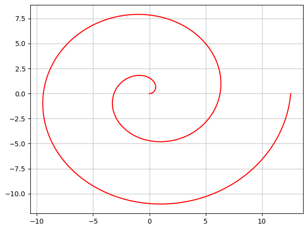
<spb.backends.matplotlib.matplotlib.MatplotlibBackend at 0x7f66fc861e10>

With just one input variable \(u\), the Jacobian matrix of \(\boldsymbol r\) has just one column:

rd = r.jacobian([u])
rd

\[\begin{split}\displaystyle \left[\begin{matrix}- u \sin{\left(u \right)} + \cos{\left(u \right)}\\u \cos{\left(u \right)} + \sin{\left(u \right)}\end{matrix}\right]\end{split}\]

Note that with just one variable, the partial derivatives are just ordinary derivatives. Therefore, the .jacobian command is not needed as we can simply differentiate the vector function directly with the usual .diff command, which will be carried out on each entry when used on a vector:

rd = diff(r,u)
rd

\[\begin{split}\displaystyle \left[\begin{matrix}- u \sin{\left(u \right)} + \cos{\left(u \right)}\\u \cos{\left(u \right)} + \sin{\left(u \right)}\end{matrix}\right]\end{split}\]

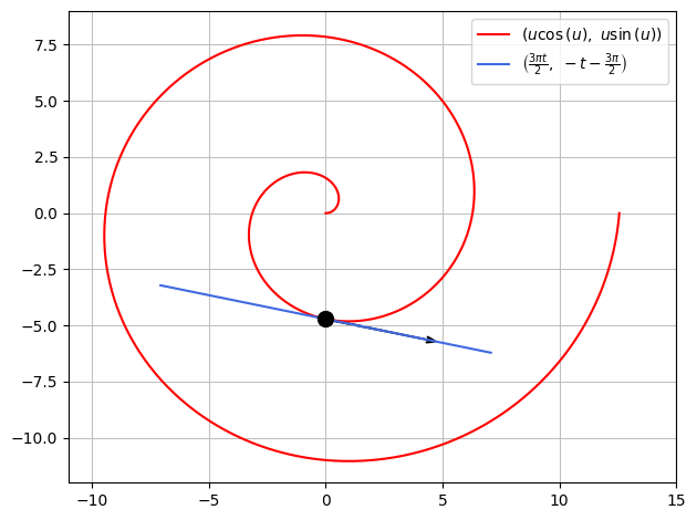
With \(\boldsymbol r\) as a parameter curve, its Jacobian matrix is in fact a tangent vector to the curve. Let us use this to construct the tangent line to the spiral at \((0,-\frac{3\pi}{2})\). This point corresponds to the parameter value \(u_0 = \frac{3\pi}{2}\):

u0 = 3*pi/2
ru0 = r.subs(u,u0)
ru0

\[\begin{split}\displaystyle \left[\begin{matrix}0\\- \frac{3 \pi}{2}\end{matrix}\right]\end{split}\]

The tangent vector from this point is thus:

rdu0 = rd.subs(u,u0)
rdu0

\[\begin{split}\displaystyle \left[\begin{matrix}\frac{3 \pi}{2}\\-1\end{matrix}\right]\end{split}\]

We can now plot this tangent vector as is, or we can construct the full tangent line with a parametric representation:

t = symbols('t', real=True)
T = ru0 + t*rdu0
T

\[\begin{split}\displaystyle \left[\begin{matrix}\frac{3 \pi t}{2}\\- t - \frac{3 \pi}{2}\end{matrix}\right]\end{split}\]

A combined plot is as follows:

p = dtuplot.plot_parametric(r[0], r[1],(u,0,4*pi),rendering_kw={"color":"red"},use_cm=False,show=False)
p.extend(dtuplot.plot_parametric(T[0],T[1],(t,-1.5,1.5),rendering_kw={"color":"royalblue"},use_cm=False,show=False))
p.extend(dtuplot.scatter(ru0,rendering_kw={"markersize":10,"color":'black'}, show=False))
p.extend(dtuplot.quiver(ru0,rdu0,rendering_kw={"color":"black"},show=False))
p.xlim = [-11,15]
p.ylim = [-12,9]

p.show()