Welcome to Sympy!#
This page provides a brief recap of the use of Sympy. If you already know Sympy, then you can skip this page and continue to the demo for semester week 1. On the other hand, if you’d like a more detailed and in-depth walkthrough of Sympy, then we will refer to this demo from the Math1a course.
Sympy is a Python library that will help out in calculations and mathematical work during the semester of Mathematics 1b.
Sympy is an abbreviation of “Symbolic Python”. In Python, loading the package sympy will allow Python to use symbolic variables and solve symbolic equations. We will also be introducing other packages when necessary. This is not intended as a guide in fundamental Python programming, but we will touch upon most tools needed for solving and visualizing mathematical problems and tasks both in theoretical, applied, and engineering-related use.
Sympy is imported and prepared for printing mathematics via the following code lines - we will start out with these lines at the top of all Sympy demos:
from sympy import *         # Import the entire Sympy package
from dtumathtools import *  # Import the dtumathtools package for plotting
init_printing()             # Initialize pretty LaTeX output
Symbolic and Numerical Variables#
Python (without Sympy) performs computations numerically. This means that all numbers and variables must be represented by a finite number of 0’s and 1’s. The study of numerical mathematics within computers is left for other courses but it is useful to be aware of unexpected situations that might arise due to this.
For example, we can all agree that
Even so, Python does not always agree with this:
0.3-(0.2+0.1)

We do not get exactly \(0.0\), and if we ask whether this is equal to \(0.0\), we get
0 == 0.3-(0.2+0.1)
False
So, we should be careful when checking whether numerical expressions are identical if we use decimal numbers.
Many of such problems can be avoided by letting Sympy take care of the maths! Use S(number) on either the numerator or denominator, or use Rational(numerator, denominator), and you will see the mathematics being handled properly by Sympy:
Rational(3,10)-(S(2)/10 + 1/S(10))

Rational(3,10)-(S(2)/10 + S(1)/10) == 0
True
We also need to be able to solve equations such as
Equations like this one can be solved using symbolic variables from Sympy. A Python variable can be created symbolically by use of one of the commands Symbol() or symbols(). Assumptions to the variables can be preset by adding a fitting argument to the command, such as \(x\in \mathbb{Z}\) with integer=True, \(x\in \mathbb{C}\) with complex=True (the default), and \(x\in \mathbb{R}\) with complex=False or real=True. A few examples:
x = symbols('x', complex=True)
3*x**2-x

l, p, t = symbols('lambda, phi, theta', real=True)
t**2 + sin(l)/tan(p)

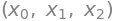
x_list = symbols('x0:3')
x_list
With symbolic expressions we can solve equations using solve() or (better) solveset().
solveset(3*x**2-x)

Note that \(3x^2 - x\) is an expression and not an equation to be “solved”. When solve and solveset are called with just an expression and nothing more, Python will by default add a right-hand side of \(0\), meaning we are actually solving the equation \(3x^2-x=0\) above. With a non-zero right-hand side, the equation ought to first be created with the command Eq(left-hand side,right-hand side):
my_equality = Eq(3*x**2-x, p+27)
my_equality

Since the equation has multiple unknowns (symbols), we have to tell with respect to which variable Python should solve the equation:
solveset(my_equality, x)

Functions and Plots#
Sympy has a large library for both functions and plots. Let us here briefly show a few examples of plotting.
plot(x**2-x+3)
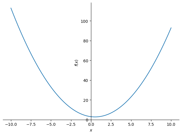
<sympy.plotting.backends.matplotlibbackend.matplotlib.MatplotlibBackend at 0x7f73256bd110>
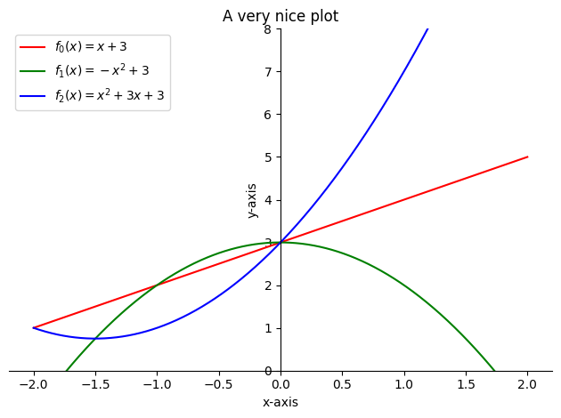
Your plots are customizable to a large extend:
p = plot(x+3,-x**2+3,x**2+3*x+3, (x,-2,2), show=False)
p[0].line_color = 'red'
p[1].line_color = 'green'
p[2].line_color = 'blue'
p.xlabel = "x-axis"
p.ylabel = "y-axis"
p.title = "A very nice plot"
p[0].label = '$f_0(x)=x+3$'
p[1].label = '$f_1(x)=-x^2+3$'
p[2].label = '$f_2(x)=x^2+3x+3$'
p.legend = True
p.ylim = (0,8)
p.show()
We will be covering plots much more in the upcoming demos.
Additional Hints#
Below follow a couple of hints that will ease and improve your use of Sympy and Jupyter Notebooks.
Markdown and Code#
As already shown, in a Jupyter Notebook you can write in two different modes: Markdown and Code. When focused on a Code cell, you are working in Python. You can insert as many lines as you wish within a cell. The last line in a cell will be printed, if it is printable.
y = Symbol('y', complex=True)
sqrt(y**2+2)

Write several things in the last line in a cell, and they will all be printed (if printable) in a comma-separated fashion:
expression = sqrt(y**2+2)
expression, expression.subs({y:2/3}) <= 1.6

A cell is executed (or run) with the keyboard shortcut Ctrl+Enter or Shift+Enter (with the latter, the focus is moved to the next cell).
Always keep in mind that all code cells that are run are “remembered”, regardless of the order in which they are placed in the document. This means that running earlier cells further up in the document one more time can risk resulting in unexpected outputs. For example:
y ** 2

# When you have run this cell, then try running the previous cell again
y = 2
It is worthwhile to mention that Python commands might not work properly and might throw an error if used wrongly (e.g. with wrong arguments or syntax errors) and sometimes when there is no solution to what you are trying to do. (Sometimes, though, this is exactly what you wants to show.) For example, if a symbol cannot be transposed, an error will be displayed:
y = Symbol('y')
y.Transpose()
---------------------------------------------------------------------------
AttributeError                            Traceback (most recent call last)
Cell In[18], line 2
      1 y = Symbol('y')
----> 2 y.Transpose()

AttributeError: 'Symbol' object has no attribute 'Transpose'
We can “catch” and handle this error more neatly with a try/except structure:
try:
    y.Transpose()
except:
    print("Symbols cannot be transposed!")
Also use this to avoid the issue of, e.g., a script file breaking and no more code being run when an error is thrown.
Helpful Tips#
Restart: If you want Python to forget all saved variables, such as when y is given the value 2, you must restart the kernel (look for something like “main Notebook Editor toolbar” in VS Code right above the editor window). “Clear Outputs” in VS Code will remove all outputs without clearing the memory.
Keyboard shortcuts: When using VS Code, an essential keyboard shortcut is Ctrl+Shift+P (on Mac: ⇧⌘P). This opens the search function for commands. Now simply type what you need when you e.g. want to create a new cell, execute the whole document, or create a new file. You can easily add custom keyboard shortcuts for your often-used tools.
Keyboard shortcuts that we have found particularly useful in the making of these demos are:
Create new cells (simply search for insert cell below)
Change a cell from Code to Markdown (change cell to code and change cell to markdown)
Restart notebook and run all cells from top down (restart the kernel, then re-run the whole notebook)
Latex: In these demos you will see examples of pretty formatting of mathematics in and between text lines. This is done using LaTeX code, a markdown syntax we highly recommend that you learn for your own scientific writing of reports, assignments, and projects. Writing mathematics inline with text is done by wrapping the latex code in Dollar signs $...$, and for a centred large version of, e.g., an equation on its own new line, then use a latex environment like \begin{equation}...\end{equation}, or simply $$...$$.
Functions: It can be of good use to know about Python functions. If a series of steps are to be carried out to solve an exercise, and the same exercise repeats with different numbers, then it is useful to think like a programmer and create a Python function for it. Examples of this will be shown in the demos where relevant. So, if there is no built-in function that can do your task for you, then just create your own Python function!
Links#
These demos are designed to include what is most useful and here and there what is nice to have for following the Mathematics 1b course. If anything is unclear or you would like to know more about particular commands or Python functions, then refer to the documentation where you can search for the topic or command. The three most important links are:
Covering the basics (variables, functions, and more): https://docs.sympy.org/latest/modules/core.html
About matrices: https://docs.sympy.org/latest/modules/matrices/matrices.html
About plotting: https://docs.sympy.org/latest/modules/plotting.html