Demo 7: Riemann Integrals#
Demo by Karl Johan Funch Måstrup Kristensen, Magnus Troen, and Jakob Lemvig. Revised March 2026 by shsp.
from sympy import *
from dtumathtools import *

init_printing()
For integration work there is no avoiding Sympy’s integrate() command. The first two sections of this demo will show the use of this command for finding antiderivatives and definite integrals.
In more advanced cases of integration, though, integrate() can run into difficulties with an integral. Then you will have to use your knowledge from the course to make the expression more “edible” for Sympy; sometimes Sympy needs it cut into smaller pieces to not suffocate, other times it needs an alternative approach entirely, possibly even a numerical approach. The final two sections will show some approaches to how we can handle such integrals that are too advanced for being solved with integrate() directly.
Integration in One Dimension#
The Indefinite Integral (Antiderivatives)#
As the textbook details, an antiderivative of a function \(f\) is any function \(F\) that fulfills \(\mathrm dF(x)/\mathrm dx=f(x)\), written with integration notation as:
Remember that adding a constant to any antiderivative results in another antiderivative. Adding an arbitrary constant to any antiderivative produces an expression for all antiderivatives (what we often call the indefinite integral), \(F(x)+c\,,\,c\in\Bbb R\).
As an example, let’s integrate a function \(f:\mathbb{R} \to \mathbb{R}\) given by
x = symbols("x", real=True)
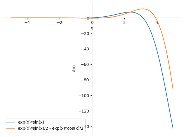
f = exp(x)*sin(x)
f

Sympy will give you the smallest antiderivative (the one without any added constant) with the command integrate(integrand, variable). Note that the variable argument can be left out when the function only has one variable.
F = integrate(f, x)
F

plot(f, F, (x,-5,5), legend=True)
<sympy.plotting.backends.matplotlibbackend.matplotlib.MatplotlibBackend at 0x7fbcf5628ad0>
As mentioned, Sympy does not add constants after an integration. You can always add an arbitrary constant \(C\in\Bbb R\), manually, if you need the full indefinite integral that represents all antiderivatives:
C = symbols('C')
F = integrate(f, x) + C
F

A Definite Integral#
A definite integral over an interval \([a,b]\subset \Bbb R\) is, according to the fundamental theorem of calculus (see the textbook), the difference in any antiderivative evaluated at the two points \(a,b\):
We often refer to this value as “the area under the graph” in the interval. Let’s say we seek to calculate:
With Sympy, simply add the interval end points to the command: integrate(integrand, (variabel, a, b)):
integrate(f, (x, -1, 1)) , integrate(f, (x, -1, 1)).evalf()

Alternatively, since we have already calculated an antiderivative, we can manually do the subtraction:
F.subs(x, 1) - F.subs(x, -1)

Integration in Multiple Dimensions#
When working with functions of multiple variables you will often see repeated integrations being required (when dealing with axis-parallel regions e.g.). A double integration,
can be determined by Sympy with integrate(integrand, x1, x2). If you seek a definite integral over given intervals on the variables,
simply add more variable tuples in the command with the syntax integrate(integrand, (x1, a1, b1), (x2, a2, b2)).
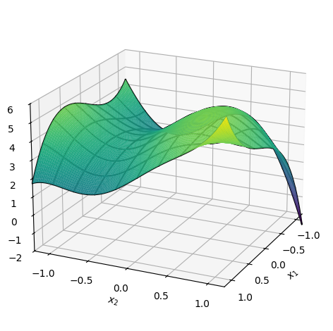
Let us consider a function \(f:\Bbb R^2\to\Bbb R\) given by \(f(x_1,x_2)=(x_1x_2)^3 - x_1^2 + \sin(3 x_2) + x_1x_2^2 + 4\):
x1, x2 = symbols('x1 x2')
f = (x1*x2)**3 - x1**2 + sin(3 * x2) + x1*x2**2 + 4
f

p = dtuplot.plot3d(f, (x1, -1.2, 1.2), (x2, -1.2, 1.2), zlim=(-2, 6), use_cm=True, colorbar=False,
                   camera = {'azim': 25, 'elev': 20}, wireframe=True)
The indefinite integral is, for \(C\in\Bbb R\):
integrate(f, x1, x2) + C

A definite integral would in the case of two variables correspond to “the volume under the graph”. The definite integral in, for instance, the region \((x_1,x_2)\in[-1.2,1.2]^2\) is:
integrate(f, (x1, -1.2, 1.2), (x2, -1.2, 1.2))

Tips and Tricks for making Sympy Integrate#
When Sympy runs into problems with an integral, here are some tricks that often will help. Such problems can result in Sympy not giving a useful result or in Sympy spending far too long on a computation, possibly without ever finishing.
Define Variables with Constraints/Assumptions#
Give Sympy information about the variables you define when you define them as symbols. Is it, say, a positive real variable, then tell that to Sympy. The most useful of such constraints are:
real = Truepositive = Truenegative = Truenonnegative = Truenonzero = True
Some examples:
x1 = symbols('x1', real = True, nonnegative = True) # x1 is real and non-negative
x2 = symbols('x2', nonzero = True) # x2 is different from zero
Simplify before Integrating#
Calling simplify on the integrand before integrating can in many cases reduce the time required for Sympy to integrate.
The work flow could look like this:
x1, x2 = symbols('x1 x2',real=True)
f = 1 / (x1 + x2)

integrand = simplify(f)
F = integrate(integrand, x1, x2)
F

Make Use of the Linearity of Integrals#
In order to integrate the expression
it will often be to your advantage to first rewrite to:
Performing the integration is now done in two steps after which you must manually put everything together. As an example, let’s compute:
x,y = symbols('x y')
f = S(27)/3 * cos(x) - 4 * atan(y -x)

# The integral limits
a = 3
b = 10
c = 2
d = 5
If you try to let Sympy compute the entire integral in one go as in the following code line, you might soon run out of patience and you will then need to stop the Python kernel in VS Code to end the computation, or maybe Sympy will simply refuse to produce a result.
#integrate(f, (x, a, b), (y, c, d)) # Don't run this line unless you want to see the issue
So, instead of doing that, let’s split the integration by making use of the lineary, resulting in two smaller integrals:
integrand1 = simplify(cos(x)) # Here it is actually not necessary to use simplify
integrand2 = simplify(atan(y - x))

F = S(27)/3 * integrate(integrand1, (x, a,b), (y, c,d)) - 4 * integrate(integrand2, (x, a,b), (y, c,d))
F

Let’s evaluate this as a decimal number for a useful result:
F.evalf()

Find an Antiderivative First and Insert Limits Next#
Sometimes Sympy won’t evaluate a definite integral:
f = tan(ln(x**2))**3 / x

integrate(simplify(f), (x,3,10))

But it can find an antiderivative:
F = integrate(f, x)
F

Thus, we can get around the issue by manually calculating the definite integral via the fundamental theorem of calculus:
F_definite = F.subs(x, 10) - F.subs(x, 3)
F_definite

F_definite.evalf()

Use the .doit() Command#
If Sympy gives an output with a non-finished integration, we can in some cases force Sympy to evaluate the integral using integrate(integrand, (variable,a,b)).doit(). This risks resulting in an error, though, but it can be worth a try.
Numerical Methods#
In some cases Sympy still spends an incredibly long time or cannot find a result for an integral even after you have helped it out as much as you can. In such cases you might have no other choice than to solve the integral numerically. Methods for that require numerical libraries such as Numpy and Scipy. If you haven’t installed these already, e.g. for use in other courses, then do it now via a terminal (note that dtumathtools automatically installs the numpy package):
# conda install scipy # If you use pip3, then type pip instead of conda
The Scipy library contains the commands quad, which is a numerical integrator for functions of one variable, and nquad, which is a numerical integrator for functions of multiple variables. Let’s fetch these and use them in the following subsections:
from scipy.integrate import quad, nquad
import numpy as np
Numerical Integration in One Dimension#
Let us have a look at the integral
f = tan(ln(x**2))**3 / x

integrate(f, (x,pi,10))

Sympy won’t evaluate the integral, so we will try to find a numerical solution.
Firstly we will convert \(f\) to a Python function, specifically a lambda function. This is done with the command lambdify, which is, roughly speaking, a shortcut to defining \(f\) with def f(x)::
f_num = lambdify(x, f, 'numpy')
f_num(3)

Such a numerically-defined function cannot be displayed with its functional expression (i.e., typing f_num will produce an error, even if you defined x as a symbol first). But we can evaluate it at chosen points, as done above at 3.
Now, quad can be used to determine the integral numerically:
F_num, error = quad(f_num, np.pi, 10)
F_num, error

Note that it is important that we use Numpy’s version of \(\pi\), which is why we typed np.pi.
The function quad provides two outputs: First, the numerical approximation of the integral; next, an estimated error (deviation) from the exact solution.
Now, this particular function is actually one of those cases where Sympy is able to find an analytical solution if we just help out a bit. Let us try to compare the numerical solution with an analytical solution. We can start out by attempting to force Sympy to evaluate the integral with .doit() - but that just returns an error:
# integrate(f, (x, pi, 10)).doit() # Remove # to see the error yourself.
As another attempt, let’s see if Sympy will produce an antiderivative which we then can manually calculate the definite integral with:
F_ad = integrate(f, x)
F_ad
F_analytic = trigsimp(F_ad.subs(x,10) - F_ad.subs(x,pi))
F_analytic

It worked! (The trigsimp command is a trigonometric simplifier that forces trigonometric terms to cancel out and reduce when possible via some trigonometric relations.)
Let us compare the two results:
F_analytic.evalf() - F_num

It is clear that the numerical solution gives a fairly good approximation, but the two results are not entirely equal. Note that the true error that quad incurs is significantly smaller than the estimated error of \(3.4 \cdot 10^{−11}\), which is not that bad.
Numerical integration in two dimensions#
As a final example, let’s consider the integration:
Here, Sympy has no problems finding a solution, so we can easily compare the analytical to the numerical method:
x,y = symbols('x y', real = True)

f = sin(x)*y**2

F_analytic = integrate(f, (y,-10,20), (x,0,pi))
F_analytic

To evaluate the integral numerically we must again define \(f\) as a Numpy function using lambdify:
f_num = lambdify((x,y), f, 'numpy')   # lambdify can take multiple variables
f_num(3,4)

Now the integral can be determined using nquad. For a function of \(n\) variables, nquad is called with the syntax nquad(funktion, [[range for variabel 1], [range for variabel 2], ..., [range for variabel n]]). In our case with two variables, we write:
F_num, error = nquad(f_num, [[0, np.pi], [-10,20]])
F_num, error

The two methods can now be compared:
F_num - F_analytic
