Week 9a: Line and Surface Integrals of Scalar Functions

Demo by Christian Mikkelstrup, Hans Henrik Hermansen, Jakob Lemvig, Karl Johan Måstrup Kristensen, and Magnus Troen

from sympy import *
from dtumathtools import*
init_printing()
x,y,z = symbols('x y z', real=True)

Curve Lengths

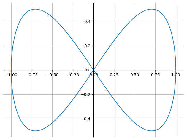
We are given a parameter curve,

u,v = symbols('u v', real=True)
r = Matrix([sin(u), sin(u)*cos(u)])
r

\[\begin{split}\displaystyle \left[\begin{matrix}\sin{\left(u \right)}\\\sin{\left(u \right)} \cos{\left(u \right)}\end{matrix}\right]\end{split}\]

where \(u \in [0, 2\pi]\).

p_curve = dtuplot.plot_parametric(*r, (u,0,2*pi), use_cm=False, label="r(u)",axis_center="auto")

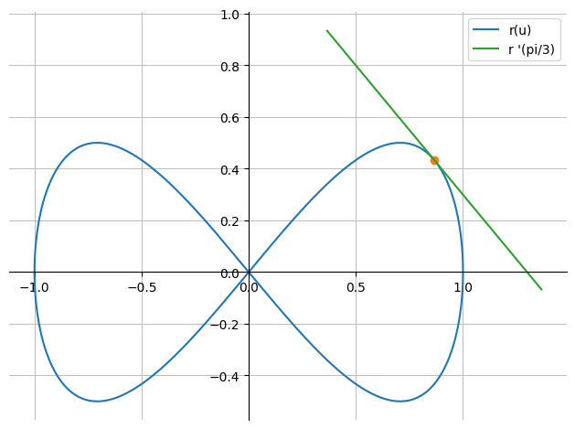
Tangent Vector and Tangent

We find the tangent vector,

dr = r.diff(u)
dr

\[\begin{split}\displaystyle \left[\begin{matrix}\cos{\left(u \right)}\\- \sin^{2}{\left(u \right)} + \cos^{2}{\left(u \right)}\end{matrix}\right]\end{split}\]

We now find the parametric representation for the tangent corresponding to the curve point \(r(\pi/3)\),

t = symbols("t")
r_tan = r.subs(u,pi/3) + t*dr.subs(u,pi/3)
r_tan

\[\begin{split}\displaystyle \left[\begin{matrix}\frac{t}{2} + \frac{\sqrt{3}}{2}\\- \frac{t}{2} + \frac{\sqrt{3}}{4}\end{matrix}\right]\end{split}\]

p_point = dtuplot.scatter(r.subs(u,pi/3), show=False)
p_tan = dtuplot.plot_parametric(*r_tan, (t,-1,1), use_cm=False, label="r '(pi/3)", show=False)


(p_curve + p_point + p_tan).show()

Length of the Curve

And then the length of this curve can be found by

\[\begin{equation*} \int_K\; \mathrm{d}\pmb{s} = \int_{0}^{2\pi} \Vert r'(u) \Vert \mathrm{d}u \end{equation*}\]

Jacobian = dtutools.l2_norm(dr)
integrate(Jacobian, (u,0,2*pi)).n()

Line Integral in 3D space

We are given a function:

x,y,z = symbols("x y z")
f = lambda x,y,z: sqrt(x**2 + y**2 + z**2)
f(x,y,z)

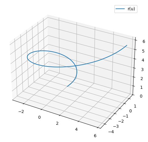
and a parameter curve (a so-called space curve)

r = Matrix([u*cos(u), u*sin(u), u])
r

\[\begin{split}\displaystyle \left[\begin{matrix}u \cos{\left(u \right)}\\u \sin{\left(u \right)}\\u\end{matrix}\right]\end{split}\]

for \(u\in[0,5]\).

p_spacecurve = dtuplot.plot3d_parametric_line(*r, (u,0,2*pi), use_cm=False, label="r(u)",aspect="equal", legend=True)

The restriction of the function to the curve is:

restriction = f(*r).simplify()
restriction

and if one remembers that \(u\) is positive, since we have defined \(u\in [0, 5]\), then the absolute value is irrelevant. From the definitions of our u and v we do though have them defined by

u,v = symbols('u v', real=True)

where SymPy only takes into account the assumption that \(u=|u|\) in exactly this case. If we had defined them using

u,v = symbols('u v', real=True, nonnegative=True)

instead, we could have used \(\verb|refine()|\) and \(\verb|Q.|\textit{assumption}\verb|(symbol)|\), where assumption can be replaced by the entries in this table.

We shall here use \(\verb|Q.nonnegative()|\), and then SymPy shows that the restriction in fact is

true_restriction = refine(restriction, Q.nonnegative(u)) # Q.nonnegative(u) tells refine() that u >= 0
true_restriction

for \(u \in [0,5]\). Whether we write \(u\) or \(|u|\) in the expression can sometimes make a difference if SymPy tries to integrate it.

Let’s return to the line integral that we wish to compute: \(\int_K f(x,y,z)\, \mathrm{d}\pmb{s}\).

First, we find the tangent vector,

dr = r.diff(u)
dr

\[\begin{split}\displaystyle \left[\begin{matrix}- u \sin{\left(u \right)} + \cos{\left(u \right)}\\u \cos{\left(u \right)} + \sin{\left(u \right)}\\1\end{matrix}\right]\end{split}\]

The length of the tangent vector \(||r_u'(u)||\) is equal to the Jacobian,

Jacobian = dtutools.l2_norm(dr).simplify()

# The following lines only works if $u$ is a real variable
# meaning if 'u = symbols('u', real=True)':
# Jacobian = dr.norm()

Jacobian

We can now find the integral along the curve,

integrate( f(*r) * Jacobian ,(u,0,5)).evalf()

and the length of the curve,

integrate(Jacobian,(u,0,5)).evalf()

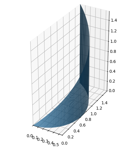
Integral over Cylinder Surface in \(\mathbb{R}^3\)

We consider a function \(f: \mathbb{R}^3 \to \mathbb{R}\) given by

\[\begin{equation*} f(x,y,z) = 8 z. \end{equation*}\]

We also consider a surface given by the following parametric representation with \(u \in [0,\frac{\pi}{2}]\) and \(v \in [0,1]\):

# This time we remember 'nonnegative=True', since we again see that
# none of the intervals for u and v contain negative numbers
u,v = symbols('u v', real=True, nonnegative=True)
r = Matrix([u*cos(u),u*sin(u),u*v])

def f(x,y,z):
    return 8*z

r, f(x,y,z)

\[\begin{split}\displaystyle \left( \left[\begin{matrix}u \cos{\left(u \right)}\\u \sin{\left(u \right)}\\u v\end{matrix}\right], \ 8 z\right)\end{split}\]

dtuplot.plot3d_parametric_surface(*r,(u,0,pi/2),(v,0,1), aspect='equal')

<spb.backends.matplotlib.matplotlib.MatplotlibBackend at 0x7f16e687f1c0>

Side Note: Interactive 3D plots

Note: This is not needed. Personally, though, we think that it is nice to be able to turn and rotate 3D plots, and have a better overview over what is happening in the plot.

Second note: Apart from that, one also must be aware that one’s notebook cannot be exported to PDF, if one has plots of this type in the document. There are work-arounds for this, but do consider whether you want to spend time on figuring it out.

If one wants to be able to move a 3D plot in order to achieve a better sense of the plot, it is an option to use another backend when plotting. This does though require that one installs the package plotly with pip:

pip install plotly

Or by removing the commenting from the cell below and execute it a single time. Then plotly will be installed in the version of Python that your notebook is using right now.

# ! pip install plotly

#                                                                           vvvvvvvvvvvvvvvvvv  her
# dtuplot.plot3d_parametric_surface(*r,(u,0,pi/2),(v,0,1), aspect='equal', backend=dtuplot.PB, use_cm=True)

The Jacobian of a Surface in 3D

We find the Jacobian and insert the parametric representation in \(f\):

crossproduct = r.diff(u).cross(r.diff(v))
Jacobian = sqrt((crossproduct.T * crossproduct)[0]).simplify()
Jacobian

integrand = f(*r) * Jacobian
integrand

integrate(integrand,(v,0,1),(u,0,pi/2)).evalf()