from sympy import *
from dtumathtools import *

init_printing()
Solution Suggestion for HW1#
Assignment 1 in Mathematics 1b
By David Thomas Hart DTU Compute
If you have any questions/corrections/improvements - davidthart03@gmail.com
Note that the following answers are not representative of the “perfect” or “ideal” student solution. It is only meant to show correct solutions to the questions.
Problem 1#
We consider \(q(x_1,x_2,x_3)=x_1^2+7x_2^2+7x_3^2+8x_1x_2-8x_1x_3+4x_2x_3+x_1-2x_2+3\).
a)#
We want to represent \(q\) in matrix form:
\(q(x_1,x_2,x_3)=\vec{x}^TA\vec{x}+\vec{b}^T\vec{x}+c\)
where \(\vec{x}=(x_1\:x_2\:x_3)^T\), \(\vec{b}=(1\:-2\:\:0)^T\), \(c=3\) and most importantly,
\( A=\begin{bmatrix} 1 & 4 & -4 \\ 4 & 7 & 2 \\ -4 & 2 & 7 \end{bmatrix} \)
We will find the eigenvalues and eigenvectors:
A = Matrix([[1, 4, -4], [4, 7, 2], [-4, 2, 7]])
ev = A.eigenvects()
ev
We know that \(A\) is hermitian as it is real and symmetric. Therefore, we know that the eigenvector corresponding to \(\lambda_1=-3\) is orthogonal to both eigenvectors associated to the eigenvalue 9. So, we only need to use Gram Schmidt on \(\vec{v}_2\) and \(\vec{v}_3\).
u1 = ev[0][2][0].normalized()
[u2, u3] = GramSchmidt([ev[1][2][0], ev[1][2][1]], orthonormal=True)
u1, u2, u3
Let’s us check that \(\beta=\{u_1,u_2,u_3\}\) is an orthonormal basis whose associated matrix has determinant \(+1\):
U = Matrix.hstack(u1, u2, u3)
U, U.det(), U.T * U
We see that \(\beta=\{u_1,u_2,u_3\}\) is an orthonormal basis with the “usual” orientation. We can quickly check that it diagonalizes \(A\):
U.T * A * U == Matrix.diag([ev[0][0], ev[1][0], ev[1][0]])
True
b)#
We now want to find the reduced form of \(q(x_1,x_2,x_3)\). We will make use of the basis change \(\vec{x}=U\vec{y}\), substituting it into our matrix form of the expression:
y1, y2, y3 = symbols("y_1 y_2 y_3")
x = U * Matrix([y1, y2, y3])
b = Matrix([1, -2, 0])
expand((x.T * A * x + b.T * x)[0] + 3)

This matches our theory that suggests that we should have the eigenvalues as our coefficients of the square terms, and naturally we have no mixed terms either.
c)#
We want to justify that the range of \(q\) is unbounded. Since \(U\) performs an orthonormal transformation, we can just look at \(q\) in this new basis. We can consider how the function acts when we keep two of the variables constant:
This is the well-known formula for a parabola that opens downward. Similarly,
which is a parabola that opens upward. Both parabolas go through \((0,3)\), and we conclude that the image set is \(\mathrm{im}(f) = \mathbb{R}\). This clearly shows that \(q\) attains arbitrarily large and small values.
Problem 2#
Consider a function \(f:\mathbb{R}^2\rightarrow\mathbb{R}\) with the expression:
\(f(x_1,x_2)=\sin(x_1^2+x_2)+x_1-x_2+3\)
a)#
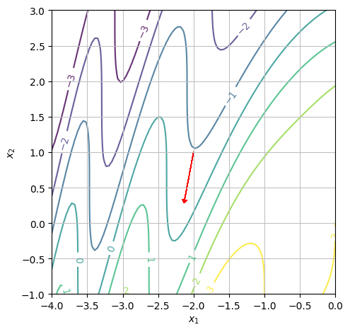
We want to display level curves and the gradient at the point \((x_1,x_2)=(-2,1)\). We can start by finding the gradient of \(f\) at the point \(P\).
x1, x2 = symbols("x_1 x_2")
f = sin(x1**2 + x2) + x1 - x2 + 3
grad = Matrix([diff(f, x1), diff(f, x2)])
# Can also be done using dtutools.gradient(f)
gradP = grad.subs({x1: -2, x2: 1})
gradP
And then generate the plot using:
zvals = [-3, -2, -1, 0, 1, 2, 3]
p1 = dtuplot.plot_vector(
    gradP,
    (x1, -2, -2),
    (x2, 1, 1),
    quiver_kw={"scale": 4, "headwidth": 8, "color": "red"},
    show=False,
    xlabel="$x_1$",
    ylabel="$x_2$",
    scalar=False,
    use_cm=False,
)
p2 = dtuplot.plot_contour(
    f,
    (x1, -4, 0),
    (x2, -1, 3),
    is_filled=False,
    show=False,
    xlabel="$x_1$",
    ylabel="$x_2$",
    rendering_kw={"levels": zvals, "alpha": 0.8},
)
(p1 + p2).show()
b)#
We want to determine whether or not the function is increasing at the point \((x_1,x_2)=(-2,1)\) in the positive \(x_1\) direction. We can see from the contour plot that \(f(-2,1)\approx-1\) and that if we continue in the positive \(x_1\) direction, the first level curve we hit is one at \(f(x_1,x_2)=0\). However, we notice that the gradient vector (red arrow) points to the left. Hence, the function is decreasing in the positive \(x_1\) direction.
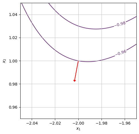
We can check this in more detail by either computing the gradient or by zooming in:
gradP.evalf()
zvals = [-0.98, -0.9589, -0, 93]
p1 = dtuplot.plot_vector(
    gradP,
    (x1, -2, -2),
    (x2, 1, 1),
    quiver_kw={"scale": 4, "headwidth": 8, "color": "red"},
    show=False,
    xlabel="$x_1$",
    ylabel="$x_2$",
    scalar=False,
    use_cm=False,
)
p2 = dtuplot.plot_contour(
    f,
    (x1, -2.05, -1.95),
    (x2, 0.95, 1.05),
    is_filled=False,
    show=False,
    xlabel="$x_1$",
    ylabel="$x_2$",
    rendering_kw={"levels": zvals, "alpha": 0.8},
)
(p1 + p2).show()
c)#
We repeat a) and b) for the point \((x_1,x_2)=(2,-1)\).
gradP2 = grad.subs({x1: 2, x2: -1})
p3 = dtuplot.plot_vector(
    gradP2,
    (x1, 2, 2),
    (x2, -1, -1),
    quiver_kw={"scale": 8, "headwidth": 8, "color": "red"},
    show=False,
    xlabel="$x_1$",
    ylabel="$x_2$",
    scalar=False,
    use_cm=False,
)
p4 = dtuplot.plot_contour(
    f,
    (x1, 0, 4),
    (x2, -3, 1),
    is_filled=False,
    show=False,
    xlabel="$x_1$",
    ylabel="$x_2$",
    rendering_kw={"alpha": 0.8},
)
(p3 + p4).show()
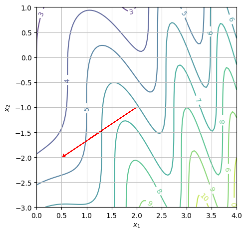
Again, we need to look at the direction of the gradient vector. Since it points to the left, function is decreasing in the positive \(x_1\) direction. The numerical value is:
gradP2.evalf()
Problem 3#
We consider two functions \(\vec{f}:\mathbb{R}^4\rightarrow\mathbb{R}^3\) and \(g:\mathbb{R}^3\rightarrow\mathbb{R}\). We are being informed that \(\vec{f}\) has the expression
\(\vec{f}(x_1,x_2,x_3,x_4)=(x_2x_3+x_1^2,-x_1x_4+x_2^3,x_1x_2x_3x_4)\).
We are furthermore informed that the Jacobian matrix \(J_g\in\mathbb{R}^{1\times3}\) of \(g\) is given by
\(J_g(y_1,y_2,y_3)=\begin{bmatrix} 1+y_3+2y_1y_2 & y_1^2+2y_2y_3^2-3 & 3+y_1+2 y_3y_2^2 \\ \end{bmatrix}\).
a)#
We want to determine \(J_{\vec{f}}(1,-2,-1,4)\).
x1, x2, x3, x4 = symbols("x1:5", real=True)
f = Matrix([[x2 * x3 + x1**2], [-x1 * x4 + x2**3], [x1 * x2 * x3 * x4]])
Jf = f.jacobian([x1, x2, x3, x4])
Jf.subs({x1: 1, x2: -2, x3: -1, x4: 4})
b)#
We now consider the composite map \(g\circ\vec{f}\). We want to evaluate the Jacobian matrix of this map in the same point as question a). Using Theorem 3.8.4, we know that \(J_{g\circ\vec{f}}(\vec{x})=J_g(\vec{y})J_{\vec{f}}(\vec{x})\). This is very neat as it means we already have all the information we need.
y1, y2, y3 = symbols("y1:4", real=True)
Jg = Matrix(
    [1 + y3 + 2 * y1 * y2, y1**2 + 2 * y2 * y3**2 - 3, 3 + 2 * y1 + 2 * y3 * y2**2]
).T
Jh = (Jg * Jf).subs({y1: f[0], y2: f[1], y3: f[2]})
Jh.subs({x1: 1, x2: -2, x3: -1, x4: 4})
Problem 4#
We are given a list of one nonzero vector \(\pmb{v}\). The idea is a append more vectors to the \(\pmb{v}\)-list. One idea could be the append a basis to the list, but SymPy’s GramSchmidt always will throw a ValueError in that case, e.g., if you call GramSchmidt([v,e1,e2,e3,e4],orthonormal=True).
The better idea is append three more linearly independent vectors to \(\pmb{v}\), and then do Gram Schmidt on the list of four vectors. Hence, the “only” difficult part of the exercise is the make sure that the vector to be appended is linearly independent to the vectors we already have.
A simple approach is:
# The standard basis of C^4:
I4 = eye(4)
e1 = I4[:, 0]
e2 = I4[:, 1]
e3 = I4[:, 2]
e4 = I4[:, 3]


# Gram-Schmidt on v, e2, e3, e4
def onb_with_v_simple(v):
    return GramSchmidt([v, e2, e3, e4], orthonormal=True)

# A complex vector v and the corresponding orthonormal basis
v = Matrix([1, 2, 2 + I, 1])
beta = onb_with_v_simple(v)
beta
# The matrix U with the vectors of beta as columns
U = Matrix.hstack(*beta)

# The matrix U is unitary:
simplify(U.H * U)
The simple approach does not work if \(\pmb{v}\) is in the span of \(\pmb{e_2},\pmb{e_3},\pmb{e_4}\) as we can see from:
u = Matrix([0, 1, 1, 0])
try:
    onb_with_v_simple(u)
except ValueError:
    print("u, e2, e3, e4 are not linearly independent")
u, e2, e3, e4 are not linearly independent
The simple approach is good enough in almost all cases since the subspace spanned by \(\pmb{e_2},\pmb{e_3},\pmb{e_4}\) is very thin set in \(\mathbb{C}^4\).
Skip the rest of the solution template for this exercise unless you are very interested in more details
It is actually not so easy to get a method that always works (and it is expected that you delivered this) and, in particular, to get a numerical stable method. The following is just Gram-Schmidt on v,e1,e2,e3,e4, where we only except \(\pmb{w}_k\) if the norm of the projection \(\pmb{w}_k\) is larger than zero (\(10^{-10}\) to account for small numerical errors):
def inner(x1: Matrix, x2: Matrix):
    """
    Computes the inner product of two vectors of same length.
    """

    return x1.dot(x2, conjugate_convention="right")


MutableDenseMatrix.inner = inner
ImmutableDenseMatrix.inner = inner
def onb_with_v(v):
    I4 = eye(4)
    e1 = I4[:, 0]
    e2 = I4[:, 1]
    e3 = I4[:, 2]
    e4 = I4[:, 3]

    # implement Gram-Schmidt
    u1 = v.normalized()

    for e in [e1, e2, e3, e4]:
        w = e - inner(e, u1) * u1
        if w.norm() > 1e-10:
            u2 = simplify(w.normalized())
            break

    for e in [e3, e4]:
        w = e - inner(e, u1) * u1 - inner(e, u2) * u2
        if w.norm() > 1e-10:
            u3 = simplify(w.normalized())
            break

    for e in [e2, e3, e4]:
        w = e - inner(e, u1) * u1 - inner(e, u2) * u2 - inner(e, u3) * u3
        if w.norm() > 1e-10:
            u4 = simplify(w.normalized())
            break

    U = Matrix.hstack(u1, u2, u3, u4)
    return U


U = onb_with_v(v)
U
U.evalf(6)
# The matrix U is unitary:
simplify(U.H * U)
A numerical stable method should probably use NumPy or a similar library:
import numpy as np

v = np.array([1, 2, 2 + 1j, 1]).reshape(4, 1)
# Use the QR decomposition instead of the Gram-Schmidt process:
U_np, _ = np.linalg.qr(v, mode="complete")
U_np
array([[-0.30151134+0.j        , -0.60302269+0.j        ,
        -0.60302269+0.30151134j, -0.30151134+0.j        ],
       [-0.60302269-0.j        ,  0.72060454+0.j        ,
        -0.27939546+0.13969773j, -0.13969773+0.j        ],
       [-0.60302269-0.30151134j, -0.27939546-0.13969773j,
         0.65075567+0.j        , -0.13969773-0.06984887j],
       [-0.30151134-0.j        , -0.13969773+0.j        ,
        -0.13969773+0.06984887j,  0.93015113+0.j        ]])
Problem 5#
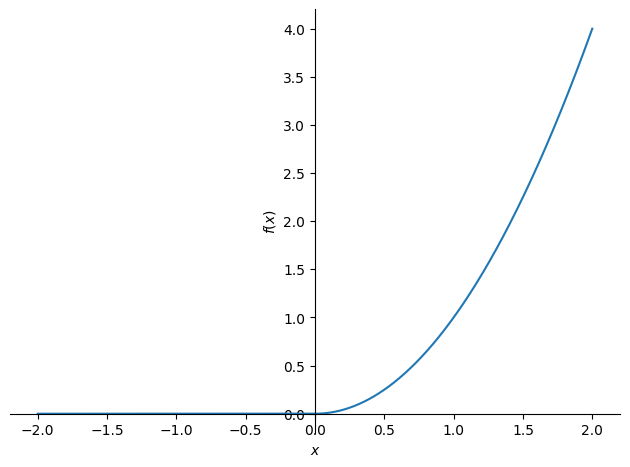
Consider a function \(f:\mathbb{R}\rightarrow\mathbb{R}\) with the expression: \(f(x)=(\text{ReLU}(x))^2\).
We start by plotting its graph:
x = symbols('x', real=True)
f = Piecewise((0, x < 0), (x**2, x >= 0))
plot(f, (x, -2, 2), ylabel='$f(x)$', xlabel='$x$')
<sympy.plotting.backends.matplotlibbackend.matplotlib.MatplotlibBackend at 0x7f2635239580>
a)#
We want to justify that \(f\) is differentiable on the entire axis and provide the expression for \(f'\). The only point where it is not obvious that the function is differentiable is \(x_0=0\). To show that the function is differentiable in \(x_0=0\), we must prove that there is a constant \(c_1\) and an epsilon function \(\varepsilon_1\) that satisfies:
Using the definition of \(f\), this is equivalent to:
We can now just “solve for \(\varepsilon_1\)”. Since we always define \(\varepsilon_1(0)=0\), we then get:
Note: To verify differentiability of the function at \(x_0\) it is not finding the expression for the epsilon-function that is difficult! We can always just rearrange the term to isolate the epsilon-function \(\varepsilon_1\). The difficulty is: Showing the requirement on \(\varepsilon_1\) which is that \(\varepsilon_1(h) \to 0\) as \(h \to 0\). A function with this property is sometimes called an “epsilon-function”.
Here that is not too difficult: If \(h<0\), then \(\varepsilon_1 (h) = (0 - c_1 h)/h = c_1\) which only goes to zero as \(h \to 0\) if \(c_1=0\). So we conclude that \(c_1=0\). Therefore our \(\varepsilon_1\) reduces to:
Recall that \(f(h) = h^2\) if \(h>0\) and \(f(h) = 0\) if \(h<0\). Hence,
which is clearly an epsilon function. Hence, \(f\) is a differentiable function and:
b)#
Let us start by plotting \(f'\) to get some intuition about where to look:
plot(f.diff(), (x, -2, 2), ylabel='$f(x)$', xlabel='$x$')
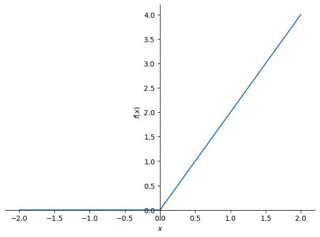
<sympy.plotting.backends.matplotlibbackend.matplotlib.MatplotlibBackend at 0x7f2635364f40>
It looks like \(f'\) is not differentiable at \(x_0 = 0\), which is further supported by:
f.diff().diff()
To prove that the function is not differentiable at \(x_0=0\), we must prove that there do not exist a constant \(c_2\) and an epsilon function \(\varepsilon_2\) that satisfy:
We can insolate \(\varepsilon_2\) and proceed as in a), or we can argue as follows: The expression above can be divided into 2 parts:
Since \(\varepsilon_2\) is an epsilon function the first expression implies that the only value of \(c_2\) possible is \(c_2 =0\), which leads to:
This can be rewritten as:
which is clearly not an epsilon function.
c)#
We want to justify that \(f'\) is continuous on the entire axis. Since \(\text{ReLU}(x)\) is continuous in \(x_0=0\), it follows that \(2\text{ReLU}(x)=f'(x)\) is continuous in \(x_0=0\).