Week 1: Preparation#
We recommend that you read the assigned textbook sections and complete the preparatory exercises before attending class. If the textbook material is challenging, even skimming the sections beforehand is very beneficial - a deeper reread can be done after class where you this time gain deeper understanding. We do not wish to discourage students from consulting additional materials to support their preparation; however, while resources such as YouTube videos may be helpful, they must not replace proper preparation using the course textbook and course material.
Reading Material#
Review: Chapter 0
Reading: Read Chapter 1 through Example 1.4.4. In Chapter 2, read Section 2.2 and the parts from Section 2.1 that concern \(\Bbb R^n\) (so, until Example 2.1.1 plus Definition 2.1.3 and Example 2.1.7). Read Chapter 3 through Section 3.3 except the parts concerning proof of differentiability (so, skip Definition 3.1.2 through Example 3.1.4).
Python: Demo 1
Key Concepts#
This week we will explore the following concepts in great detail. You are expected to have familiarized yourself with them before classes.
Long Day will cover:
Multi-variable scalar functions
Multi-variable vector functions
Graphs
Parametrizations
Continuity
Short Day will cover:
Level sets
Quadratic forms
The standard inner product (dot product) and norm in \(\mathbb{R}^n\)
Partial derivatives and the gradient vector
Preparatory Exercises#
I: The Function Value at a Point#
Question a#
Substitute the values \(x = 2\) and \(y = -1\) into the functional expression \(f(x, y) = x^2 + 3xy + 4y^2\) and calculate \(f(2, -1)\).
Hint
Substitute \(x\) with \(2\) and \(y\) with \(-1\) in the expression \(x^2 + 3xy + 4y^2\).
Answer
\(f(2, -1) = 2^2 + 3(2)(-1) + 4(-1)^2 = 4 - 6 + 4 = 2\)
Question b#
Let \(g: \mathbb{R}^2 \to \mathbb{R}\) be given by the functional expression \(g(x_1, x_2) = x_1^2 + 3x_1 x_2 + 4 x_2^2\). Calculate \(g(2, -1)\).
Hint
This is the same functional expression as in the previous question, so method and answer are the same.
Question c#
Let \(\alpha \in \mathbb{R}\). Find \(g(2 \alpha, \alpha)\) and \(g(\alpha, 2 \alpha)\), where \(g\) is the function defined in the previous question. Calculate the derivative of \(g(2 \alpha, \alpha)\) with respect to \(\alpha\).
Hint
For \(g(2 \alpha, \alpha)\), substitute \(x_1 = 2 \alpha\) and \(x_2 = \alpha\) into \(g(x_1, x_2) = x_1^2 + 3x_1x_2 + 4x_2^2\). Repeat for \(g(\alpha, 2 \alpha)\). For the derivative, differentiate the expression for \(g(2 \alpha, \alpha)\) with respect to \(\alpha\).
Answer
Substituting gives:
\(g(2 \alpha, \alpha) = (2\alpha)^2 + 3(2 \alpha)(\alpha) + 4(\alpha)^2 = (4+6+4)\alpha^2 = 14 \alpha^2\) and \(g(\alpha, 2\alpha) = (\alpha)^2 + 3(\alpha)(2\alpha) + 4(2\alpha)^2 = (1+6+16) \alpha^2 = 23 \alpha^2\).
The derivative of \(g(2 \alpha, \alpha) = 14 \alpha^2\) with respect to \(\alpha\) is \(\frac{\mathrm d}{\mathrm d\alpha} \big( 14 \alpha^2 \big) = 28 \alpha\).
II: Level Curves#
Describe the level curves (contour lines) for the function \(f: \mathbb{R}^2 \to \mathbb{R}\) given by \(f(x, y) = x^2 + y^2 - 5\).
Hint
Try to set the function equal to some randomly chosen constant, such as \(f(x, y) = 9\), for an example of a level curve. What shape does the curve have? Remember that you cannot conclude this based on just looking at the plot - you must confirm it analytically.
Hint
Do you recognize the circle equation? If you have forgotten the circle equation, then now is the time to look it up. Afterwards, set the function equal to an arbitrary constant \(c\in\Bbb R\). Can you show that all level curves are shaped as circles for all \(c>-5\)?
Hint
If you have trouble visualizing this, then use Python to plot, e.g., the level curve for \(f(x, y) = 9\):
x, y  = symbols("x y", real=True)
f = x**2 + y**2 - 5
dtuplot.plot_implicit(Eq(f,9), (x,-10,10), (y,-10,10))
III: Graph or Level Curve?#
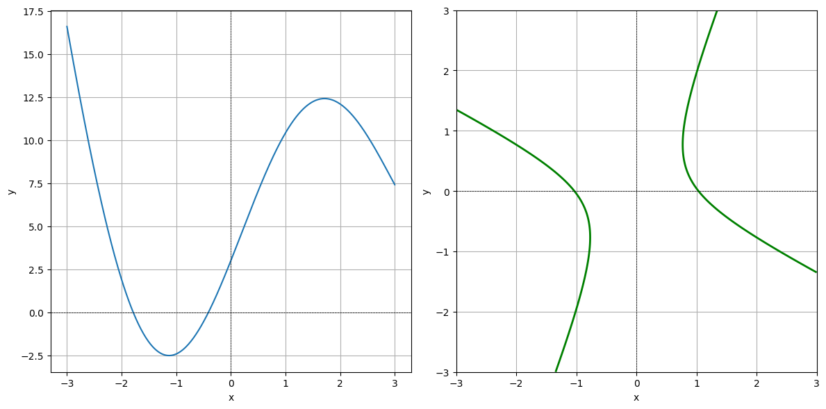
Below are shown the graph of a function \(f_1\) of one variable and a level curve of a function \(f_2\) of two variables. Which plot is the graph, and which is the level curve?

IV: Discontinuous at One Point#
Draw, describe, or define a function \(h: \mathbb{R} \to \mathbb{R}\) that is continuous at all points except for a single point.
Answer
One possible function is \(h(x) = \begin{cases} x & \text{if } x \neq 1 \\ 0 & \text{if } x = 1 \end{cases}\). This function is continuous everywhere except at \(x = 1\).

