Demo 5: Taylor Approximations

Demo by Christian Mikkelstrup, Hans Henrik Hermansen, Jakob Lemvig, Karl Johan Måstrup Kristensen, and Magnus Troen. Revised March 2026 by shsp.

from sympy import *
from sympy.abc import x,y,z,u,v,w,t
from dtumathtools import *
init_printing()

Taylor Polynomials in One Variable

In Sympy, a Taylor expansion is performed with the command series(function, variable, expansion point, degree+1) or equivalently function.series(variable, expansion point, degree+1). To approximate \(\cos(x)\) by a sixth-degree Taylor polynomial with the expansion point \(x_0 = 0\), we write:

series(cos(x), x, 0, 7)

Note how an approximating polynomial of degree 6 is obtained by typing 7 as the last argument in the series command. Generally, you must type the desired degree plus 1 into this command, which might be surprising and is very important to remember. The technical reason is that the output, as you can see above, does not only contain the approximating polynomial but also a remainder term, which in this form always will be of one higher order than the degree of the polynomial. It is this remainder term order that the series command requires as an argument.

“Big O” Notation

The remainder term shown in this output might look unfamiliar. The textbook presents remainder terms as either epsilon functions or (Laplace) remainder function, which you will become familiar with in this course, but here we see so-called “Big O” notation, which for Taylor polynomials of degree \(K\) will have the form \(O(x^{K+1})\). This is simply an error indicator with a different purpose than the others.

Where, e.g., the remainder function can be used for estimating the incurred error, “Big O” rather tells something about the growth rate of the error. In more details, “Big O” provides an upper bound for the growth rate of the error as you move farther away from the expansion point. The output above tells that the error between the value of the approximating polynomial we have obtained and the original function \(\cos(x)\) stays below \(x^7\). Alternatively, think of it as telling you that as you approach the expansion point, the error diminishes towards zero faster than \(x^7\) would.

In this course we generally do not study the growth rate of the incurred error, so to only receive the Taylor polynomial without remainder information, remove the \(O(x^{K+1})\) term with .removeO():

series(cos(x), x, 0, 7).removeO()

Example with sin(x)

Consider the function \(f(x)=\sin(x)\) approximated from expansion point \(x_0 = 0\).

Let’s first plot \(f(x)\) along with some chosen approximating polynomials. We use the argument show = False such that we can add more plots to the plotting window with .extend() before showing the result:

pl = plot(sin(x),xlim = (-3,3), ylim = (-3,3), show=False, legend = True)
for K in [0,1,2,3,6]:
    newseries = series(sin(x),x,0,K+1).removeO()
    display(Eq(Function(f'P_{K}')(x), newseries))
    newplot = plot(newseries,label = f"n = {K}", show=False)
    pl.extend(newplot)
pl.show()

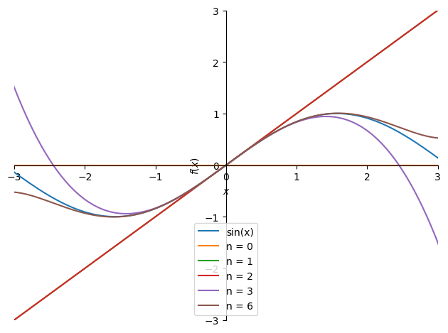
The combined plot clearly shows that by increasing the degree \(K\), we obtain a better and better approximation. Note that some approximations overlap:

\[\begin{align*} P_1(x) &= f(x_0) + f'(x_0)(x-x_0)\\ &= \sin(0) + \cos(0) x \\ &= x \\ P_2(x) &= f(x_0) + f'(x_0)(x-x_0) + \frac{1}{2} f''(x_0)(x-x_0)^2 \\ &= \sin(0) + \cos(0) x - \sin(0) x^2 \\ &= x \end{align*}\]

for \(x\in\mathbb{R}\).

Error Estimation

We wish to find the function value \(\ln\left(\frac{5}{4}\right)\), but this can be a hassle to calculate accurately (in particular if we have to find many of such values). Let us make it easier by instead using an approximating polynomial \(P_3(x)\) expanded from the point \(x_0=1\):

x = symbols("x")
P3 = series(ln(x),x,1,4).removeO()
P3

We can now use this approximation to find an approximate value of \(\ln(x)\) at \(x=\frac{5}{4}\):

val = P3.subs(x,Rational(5/4))
val, val.evalf()

So, \(\ln\left(\frac{5}{4}\right)\approx 0.224\). But how accurate is this? How large an error do we incur by using this approximate value in place of the true function’s value? Let’s do an investigation.

Maximizing the Remainder Function

The textbook tells us that a \(\xi \in \,\,]\,x_0\,,\,x\,[\) exists such that the error can be written as a remainder function \(R_n(x)\):

\[\begin{equation*} R_n\left(x\right) = \frac{f^{(n+1)}(\xi)}{(n+1)!}\cdot\left(x - x_0\right)^{n+1}. \end{equation*}\]

This remainder function represents the incurred error from using the approximation instead of the real function. Wrap it in absolute value bars, \(|R_n(x)|\), and it represents the numerical error (without sign). The largest value that this (absolute value of the) remainder function can take will be an upper bound to the error. The actual incurred error might be smaller, but since we cannot find its exact value, having an upper bound is very useful information.

Let’s fill in everything we know: At \(x=\frac{5}{4}\) with \(x_0=1\), the interval for \(\xi\) is \(\xi \in \,\,]\,1\,,\,\frac{5}{4}\,[\), and the remainder function becomes:

\[\begin{equation*} R_3\left(\frac{5}{4}\right) = \frac{f^{(4)}(\xi)}{4!}\cdot\left(\frac{5}{4} - 1\right)^4. \end{equation*}\]

Let’s compute \(f^{(4)}(\xi)\):

xi = symbols("xi")
diff(ln(x),x,4).subs(x,xi)

Thus, we have:

\[\begin{equation*} R_3\left(\frac{5}{4}\right) = \frac{-6}{4!\xi^4}\cdot\left(\frac{5}{4} - 1\right)^4. \end{equation*}\]

The only unknown is \(\xi\), and it happens to be in the denominator in this case. Thus, we maximize \(\left|R_3\left(\frac{5}{4}\right)\right|\) by minimizing \(\xi\). In its interval we thus choose the smallest possible value, so \(\xi=1\), which we substitute in:

R3 = abs(diff(ln(x),x,4).subs(x,1) * (5/4 - 1) ** 4 /(factorial(4)))
Eq(Function('R_3')(S('5/4')), R3)

Here we have an upper bound of the (numerical) error. The true (numerical) error will be below this value. If needed, we can form an error interval with the end points:

Interval(val - R3, val + R3)

In conclusion, we can guarantee that the true value of \(\ln(\frac{5}{4})\) is somewhere in the interval \(]0.2229;0.2250[\) (this is an open interval, due to rounding). As an interesting check, let’s ask Python to calculate the true value of \(\ln(\frac{5}{4})\) to confirm that it indeed is within our obtained error margin from the approximate value:

ln(5/4), Interval(val - R3, val + R3).contains(ln(5/4))

Note that even Python’s value of \(\ln(\frac{5}{4})\) is an approximation, just a much better one than ours. But we could improve our approximation by simply doing higher-degree Taylor expansions.

Limit Values using Taylor’s Limit Formula

We will now use Taylor’s limit formula to determine the limit value of different expressions. This is often usable for fractions where the numerator, denominator, or both contain expressions that are not easy to work with. For example, it is not easy to see what value the expression \(\frac{\sin(x)}{x}\) goes towards for \(x\rightarrow 0\) since both the numerator and the denominator contain \(x\).

The way to access Taylor’s limit formula in Sympy is again with the series command, but this time we will not use .removeO() since we need to keep a remainder expression. Note that the course textbook presents Taylor’s limit formula using epsilon functions for this remainder, whereas Sympy uses the “Big O” notation as explained above. To convert Sympy’s output to the epsilon format manually, we will replace “Big O” notation such as \(O(x^{K+1})\) with \(\varepsilon(x) \, x^{K}\), where \(\varepsilon(x) \to 0\) for \(x \to 0\).

Example 1

We wish to investigate the limit value of the expression \(\frac{\sin(x)}{x}\) for \(x\rightarrow 0\). Let us do a Taylor expansion to the 2nd degree of the numerator:

series(sin(x),x,0,n=3)

Note that such a Taylor expansion is identical to the true function and not just an approximation of it (because the remainder is included). We can thus replace the function by its Taylor expansion, suddenly allowing us to reduce further and find the limit value:

\[\begin{gather*} \frac{\sin(x)}{x} = \frac{x + \epsilon (x) \cdot x^2}{x} = 1 + \varepsilon (x)x \rightarrow 1, \text{ when } x \rightarrow 0. \end{gather*}\]

This works because we started out with a polynomial term in the denominator, and via a Taylor expansion we converted the numerator to polynomial terms as well (plus an epsilon function). The terms thus had a chance to cancel out and the fraction to reduce further until we, in this case, no longer had an \(x\) in both the numerator and the denominator.

Example 2

How did we know of which degree to do the Taylor expansion in the previous example? It can sometimes feel like guesswork to choose the degree that produces just the right number of just the right terms.

Consider this expression:

\[\begin{equation*} \frac{\mathrm e^x - \mathrm e^{-x} - 2x}{x-\sin(x)}. \end{equation*}\]

We wish to find its limit value for \(x \rightarrow 0\). This time the numerator and denominator contain more than just polynomial terms, so let’s Taylor expand the numerator and denominator separately. We will then see what happens as we include more and more terms by increasing the degrees. First, let’s expand both to the 1st degree:

T = E ** x - E ** (-x) - 2*x
N = x - sin(x)
series(T,x,0,2), series(N,x,0,2)

This is too imprecise since the Taylor expansions just become remainder terms. Substituting those into the fraction will not let us reduce it further (the epsilon functions for each Taylor expansion might be different, so they do not directly cancel out). Let’s try to the 2nd degree:

series(T,x,0,3), series(N,x,0,3)

Still too imprecise. To the 3rd degree then:

series(T,x,0,4), series(N,x,0,4)

Here we have something that we can try out. Substituting into the fraction:

\[\begin{gather*} \frac{\frac{x^3}{3}+\epsilon_1(x)x^3}{\frac{x^3}{6}+\epsilon_2(x)x^3} = \frac{\frac{1}{3} + \epsilon_1(x)}{\frac{1}{6}+\epsilon_2(x)} \rightarrow \frac{\frac{1}{3}}{\frac{1}{6}} = 2, \text{ when } x \rightarrow 0. \end{gather*}\]

The epsilon functions are labeled with indices since they strictly speaking might be different epsilon functions. But that has no influence as they both approach zero at the limit. Let’s check with Python’s limit() command:

limit(T/N,x,0)

Taylor Polynomials in Two Variables

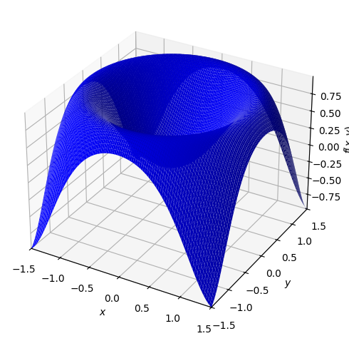
Consider the following function of two variables:

\[ f:\mathbb{R}^2 \to \mathbb{R},\quad f(x,y) = \sin(x^2 + y^2). \]

Let’s start by plotting it:

x,y = symbols("x y", real = True)
f = sin(x ** 2 + y ** 2)
dtuplot.plot3d(f,(x,-1.5,1.5),(y,-1.5,1.5),rendering_kw={"color" : "blue"})

<spb.backends.matplotlib.matplotlib.MatplotlibBackend at 0x7fe178ebcf50>

Approximating Polynomials of Different Degrees

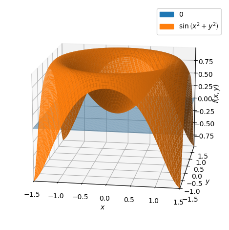
Let us determine the approximating first-degree polynomial \(P_1(x,y)\) with expansion point \((0,0)\):

P1 = dtutools.taylor(f,[x,0,y,0],degree=2)
P1

\(P_1(x,y)\) turns out to just be zero, meaning a horizontal plane at a height of zero (so, identical to the \((x,y)\) plane):

p = dtuplot.plot3d(P1,(x,-1.5,1.5),(y,-1.5,1.5),show=false,rendering_kw={"alpha" : 0.5},camera={"azim":-81,"elev":15})
p.extend(dtuplot.plot3d(f,(x,-1.5,1.5),(y,-1.5,1.5),show=False))
p.show()

With another expansion point such as \((1/10,0)\) we get:

p = dtuplot.plot3d(dtutools.taylor(f,[x,0.1,y,0],degree=2),(x,-1.5,1.5),(y,-1.5,1.5),show=false,rendering_kw={"alpha" : 0.5},camera={"azim":-81,"elev":15})
p.extend(dtuplot.plot3d(f,(x,-1.5,1.5),(y,-1.5,1.5),show=False))
p.show()

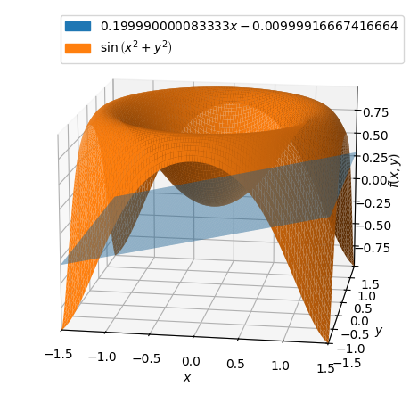
which shows that the expansion point matters a lot.

Let’s return to the expansion point \((0,0)\) and investigate the approximating second-degree polynomial:

P2 = dtutools.taylor(f,[x,0,y,0],3)
P2

dtuplot.plot3d(f,P2,(x,-1.5,1.5),(y,-1.5,1.5))

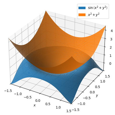
<spb.backends.matplotlib.matplotlib.MatplotlibBackend at 0x7fe176107b90>

This time, the approximating polynomial is an (elliptic) paraboloid.

Lastly, let’s go higher up in degree and have a look at the approximating 6th-degree polynomial:

P6 = dtutools.taylor(f,[x,0,y,0],7)
p = dtuplot.plot3d(f,P6,(x,-1.5,1.5),(y,-1.5,1.5),show=False)
p.legend=True
p.show()

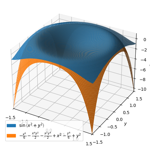
As expected, they are now much closer to each other.

Error Investigations

To see how well they fit, let us investigate the errors incurred by using our 1st-, 2nd-, and 6th-degree approximating polynomials instead of the original function to evaluate function values at different points. Let us begin at \((0.2,0.2)\):

f_p1 = f.subs([(x, 1/5), (y, 1/5)])
P1_p1 = P1.subs([(x, 1/5), (y, 1/5)])
P2_p1 = P2.subs([(x, 1/5), (y, 1/5)])
P6_p1 = P6.subs([(x, 1/5), (y, 1/5)])

error_list = (f_p1 - P1_p1, f_p1 - P2_p1, f_p1 - P6_p1)
displayable_equations = [ Eq(Function(f'P_{i}')(S('1/5')), expression) for i, expression in zip((1,2,6), error_list) ]

display(*displayable_equations)

As expected, the error is much smaller for higher-degree approximating polynomials. Let us try at \((0.5,0.5)\):

f_p2 = f.subs([(x,1/2),(y,1/2)])
P1_p2 = P1.subs([(x,1/2),(y,1/2)])
P2_p2 = P2.subs([(x,1/2),(y,1/2)])
P6_p2 = P6.subs([(x,1/2),(y,1/2)])

error_list = (f_p2 - P1_p2, f_p2 - P2_p2, f_p2 - P6_p2)
displayable_equations = [ Eq(Function(f'P_{i}')(S('1/5')), expression) for i, expression in zip((1,2,6), error_list) ]

display(*displayable_equations)

The farther away from the expansion point \((0,0)\) we go, the larger the error becomes, as expected.

Note: It should be mentioned that our comparisons are based on the assumption that Sympy’s own approximations are much better than ours. This is most likely quite a good assumption in cases like these, but it is important to know that Sympy (as well as other computer software) generally also performs approximations.

Taylor Polynomials in Three Variables

Let us in this final section leave the series command and try constructing a 2nd-order Taylor approximation (semi-)manually. For that, the course textbook provides the following formula for a second-degree Taylor polynomial of a function of multiple variables:

\[\begin{equation*} P_2(\boldsymbol{x}) = f(\boldsymbol{x}_0) + \left<(\boldsymbol{x} - \boldsymbol{x}_0), \nabla f(\boldsymbol{x}_0)\right> + \frac{1}{2}\left<(\boldsymbol{x} - \boldsymbol{x}_0), \boldsymbol{H}_f(\boldsymbol{x}_0)(\boldsymbol{x}-\boldsymbol{x}_0)\right>. \end{equation*}\]

For an example, let’s consider the function:

\[\begin{equation*} f: \mathbb{R}^3\to \mathbb{R},\quad f(x_1,x_2,x_3) = \sin(x_1^2 - x_2)\mathrm e^{x_3}. \end{equation*}\]

x1,x2,x3 = symbols('x1,x2,x3', real = True)
f = sin(x1**2 - x2)*exp(x3)
f

Let us determine the second-degree Taylor polynomial with expansion point \(\boldsymbol{x}_0 = (1,1,0)\). First, we define \(\boldsymbol{x}_0\) and \(\boldsymbol{x}\):

x = Matrix([x1,x2,x3])
x0 = Matrix([1,1,0])

Then we compute \(\nabla f(\boldsymbol{x}_0)\) and \(\boldsymbol{H}_f(\boldsymbol{x}_0)\):

nabla_f = dtutools.gradient(f,(x1,x2,x3)).subs([(x1,x0[0]),(x2,x0[1]),(x3,x0[2])])
nabla_f

\[\begin{split}\displaystyle \left[\begin{matrix}2\\-1\\0\end{matrix}\right]\end{split}\]

Hf = dtutools.hessian(f,(x1,x2,x3)).subs([(x1,x0[0]),(x2,x0[1]),(x3,x0[2])])
Hf

\[\begin{split}\displaystyle \left[\begin{matrix}2 & 0 & 2\\0 & 0 & -1\\2 & -1 & 0\end{matrix}\right]\end{split}\]

Now we have all needed components to construct the approximating 2nd-degree polynomial \(P_2\):

P2 = f.subs([(x1,x0[0]),(x2,x0[1]),(x3,x0[2])]) + nabla_f.dot(x - x0) + S('1/2')* (x - x0).dot(Hf*(x - x0))
P2.simplify()

Let’s again have a quick look at the errors we would incur by using this approximation instead of the real function at some chosen points:

v1 = Matrix([1,1,0])
v2 = Matrix([1,0,1])
v3 = Matrix([0,1,1])
v4 = Matrix([1,2,3])
vs = [v1,v2,v3,v4]

for v in vs:
    print((f.subs({x1:v[0],x2:v[1],x3:v[2]}) - P2.subs({x1:v[0],x2:v[1],x3:v[2]})).evalf())

0
0.287355287178842
0.712644712821158
-12.9013965351501

Again, we see the error increasing as we move farther away from the expansion point, as expected.