Demo 9: Plane, Volume, Line, and Surface Integrals with The Change-of-Variables Theorem

Demo by Christian Mikkelstrup, Hans Henrik Hermansen, Jakob Lemvig, Karl Johan Måstrup Kristensen, and Magnus Troen. Revised March 2026 by shsp.

from sympy import *
from dtumathtools import *

init_printing()

When integrating scalar functions over non-axis-parallel regions, such as circular discs, spheres, and curves, we cannot directly do usual Riemann-integral with respect to the variables \(x_1,\cdots,x_n\). The textbook instead gives us a technique known as the change-of-variables theorem or variable substitution that lets us push the integration over to the parameter variables instead - given that we are able to create a regular parametric representation of the region.

This demo will first treat integration over planar regions in the \((x,y)\) plane as well as through spatial regions in \((x,y,z)\) space, so, respectively, the plane integral and the volume integral. Next the demo continues with integration along curves and over surfaces, so, respectively, the line integral and the surface integral, in \(n\)-dimensional space. But before we can get started with integrations we will take a closer look at an important component in them all: the restriction of the function to the parameter region.

Restrictions to Parametrized Geometry

In order for us to integrate over our parametrized geometry with the change-of-variables theorem, we must study the component known as a restriction. Let’s consider the following scalar function \(f\) and vector function \(\boldsymbol r\):

\[\begin{equation*} f: \mathbb{R}^3 \to \mathbb{R}, \quad f(x,y,z) = x+y+z \end{equation*}\]

\[\begin{equation*} \boldsymbol{r}(u,v,w) = \begin{bmatrix} u -v \\ w^2 \\ v(u+w) \end{bmatrix}, \quad u,v,w \in \mathbb{R}. \end{equation*}\]

We wish to determine the functional composition \(f(\boldsymbol{r}(u,v,w))\). If \(\boldsymbol r\) represents a parametrized geometric region, we call this a restriction of \(f\) to \(\boldsymbol r\). What we want is for the first entry in \(\boldsymbol r\) to replace \(x\), its second entry should replace \(y\) and so on.

Let’s define \(\boldsymbol r\) as a simple vector:

u,v,w = symbols('u v w')
r = Matrix([u -v, w**2, v*(u+w)])
r

\[\begin{split}\displaystyle \left[\begin{matrix}u - v\\w^{2}\\v \left(u + w\right)\end{matrix}\right]\end{split}\]

\(f\) can be defined as either a Sympy expression (that is, stored as a simple variable), a standard Python function, or as a lambda function:

x,y,z = symbols('x,y,z', real =True)

# Sympy expression
f_sym = x+y+z 

# Standard Python function
def f_function(x,y,z):
    return x+y+z

# Lambda function
f_lam = lambda x,y,z : x+y+z

A composition like \(f(\boldsymbol{r}(u,v,w))\) is computed using different syntax depending on your choice among the above:

fr_sym = f_sym.subs(zip((x,y,z), r)).simplify()
fr_function = f_function(*r).simplify()
fr_lam = f_lam(*r).simplify()

fr_sym, fr_function, fr_lam

The Sympy expression makes use of zip, which substitutes the variables by the vector entry by entry - as a “zipper” - such that the first vector entry r[0] substitutes x, r[1] substitutes y, and r[2] substitutes z.

This is not necessary for Python functions or lambda functions. Instead, we here see the asterisk * used in front of the vector. This tells Python that the coordinates in r are to be given to the function as individual arguments.

Plane Integrals

Let’s now see an example of integration over geometry. We are given a function \(f:\Bbb R^2\to\Bbb R\) by:

\[\begin{equation*} f(x,y) = 2xy. \end{equation*}\]

f = lambda x,y: 2 * x * y
f(x,y)

Let’s reuse the parametrized circular disc \(C\) from the previous demo:

u,v = symbols('u v')
rC = Matrix([2,1]) + v * Matrix([cos(u),sin(u)])
rC

\[\begin{split}\displaystyle \left[\begin{matrix}v \cos{\left(u \right)} + 2\\v \sin{\left(u \right)} + 1\end{matrix}\right]\end{split}\]

where \(u\in [0, 2\pi] ,v\in[0, 1]\). The axis-parallel rectangle \([0, 2\pi] \times [0, 1]\) in the \((u,v)\) plane maps to the circle disc in the \((x,y)\) plane:

dtuplot.plot_implicit(((x < 2*pi) & (x > 0) & (y > 0) & (y < 1)),
                      (x, -0.5, 2*pi + 0.5), (y, -0.5,1.5),
                      title="(u,v) plane",
                      xlabel="u", ylabel="v",
                      axis_center='auto')

/builds/pgcs/pg14/venv/lib/python3.11/site-packages/spb/series.py:2255: UserWarning: The provided expression contains Boolean functions. In order to plot the expression, the algorithm automatically switched to an adaptive sampling.

<spb.backends.matplotlib.matplotlib.MatplotlibBackend at 0x7ff48d7ead50>

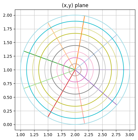
dtuplot.plot_parametric_region(
    *rC, (u, 0, 2*pi), (v, 0, 1),
    aspect="equal",
    title="(x,y) plane"
)

<spb.backends.matplotlib.matplotlib.MatplotlibBackend at 0x7ff48b78d090>

We are now tasked with computing the plane integral of \(f\) over \(C\). In mathematical notation, we are calculating:

\[\int_C f(x,y)\; \mathrm{d}\pmb{x}.\]

The circular region is not axis-parallel, so we need the change-of-variables theorem (variable substitution), which we in the textbook find this formula for:

\[\begin{equation*} \int_C f(x,y)\; \mathrm{d}\pmb{x} = \int_{0}^{1} \int_{0}^{2\pi} f(\boldsymbol r_C(u,v))\cdot|\det (\boldsymbol J_{\boldsymbol r_C}) |\;\mathrm{d}u\,\mathrm{d}v. \end{equation*}\]

The Jacobian matrix \(\boldsymbol J_{\boldsymbol r_C}\) is defined as:

\[\begin{equation*} \boldsymbol{J}_{\boldsymbol r_C} = \left[\begin{matrix} \vdots & \vdots \\ \frac{\partial \boldsymbol r(u,v)}{\partial u} & \frac{\partial \boldsymbol r(u,v)}{\partial v} \\ \vdots & \vdots \end{matrix}\right] = \left[\begin{matrix}\nabla(2 + v\cos\left(u \right))^T\\ \nabla(1 + v\cos\left(u \right))^T\end{matrix}\right]. \end{equation*}\]

JacobiM = Matrix.hstack(rC.diff(u), rC.diff(v))
JacobiM

\[\begin{split}\displaystyle \left[\begin{matrix}- v \sin{\left(u \right)} & \cos{\left(u \right)}\\v \cos{\left(u \right)} & \sin{\left(u \right)}\end{matrix}\right]\end{split}\]

The absolute value of the Jacobian determinant \(|\det(\boldsymbol J_{\boldsymbol r_C})|\) is

Jacobian = abs(det(JacobiM)).simplify()
Jacobian

This value can be thought of as a measure for how much the \((u,v)\) parameter region is deformed locally as it undergoes the map \(\boldsymbol r_C\). Our plane integral is now:

\[\begin{equation*} \int_C f(x,y)\; \mathrm{d}\pmb{x} = \int_{0}^{1} \int_{0}^{2\pi} f(2+v\cos(u),1+v\sin(u))\cdot|v|\; \mathrm{d}u \,\mathrm{d}v, \end{equation*}\]

and we will do the rest in one code line:

integrate(f(*rC) * Jacobian,(u,0,2*pi),(v,0,1))

Volume Integrals

In the previous demo we parametrized the solid unit sphere \(\Omega\) centered at the origin as follows for \(u\in[0,2\pi], v\in[0,\pi], w\in[0,1]\):

u,v,w = symbols('u v w')
r_omega = Matrix([[w*cos(u)*cos(v)],[w*sin(v)*cos(u)],[w*sin(u)]])
r_omega

\[\begin{split}\displaystyle \left[\begin{matrix}w \cos{\left(u \right)} \cos{\left(v \right)}\\w \sin{\left(v \right)} \cos{\left(u \right)}\\w \sin{\left(u \right)}\end{matrix}\right]\end{split}\]

In the following we will be doing volume integrals through this sphere. As this is not an axis-parallel region in \((x,y,z)\) space, we will need the change-of-variables theorem to push the integration over to the axis-parallel \((u,v,w)\) parameter space:

\[\begin{equation*} \int_{\Omega} f\; \mathrm{d}\pmb{x}= \int_{0}^{1} \int_{0}^{\pi}\int_{0}^{2\pi} f(\boldsymbol{r}_{\Omega})\,\,|\mathrm{det}(\boldsymbol J_{\boldsymbol r_{\Omega}})| \;\mathrm du\,\mathrm dv\,\mathrm dw. \end{equation*}\]

Finding the Sphere Volume

According to the textbook, in order to find the “size of the geometry”, which in this case of a three-dimensional sphere is its volume, the function \(f:\mathbb{R}^3 \to \mathbb{R}\) in the change-of-variables theorem should have the value \(f(\boldsymbol{x}) = 1\). This simplifies the change-of-variables formula to:

\[\begin{equation*} \mathrm{Volume}=\int_{\Omega} 1\; \mathrm{d}\pmb{x}= \int_{0}^{1} \int_{0}^{\pi}\int_{0}^{2\pi} |\mathrm{det}(\boldsymbol J_{\boldsymbol r_{\Omega}})| \;\mathrm du\,\mathrm dv\,\mathrm dw. \end{equation*}\]

The Jacobian matrix of our \(\Omega\) parametrization is

\[\begin{equation*} \boldsymbol{J}_{\boldsymbol r_{\Omega}} = \left[\begin{matrix} \vdots & \vdots & \vdots \\ \frac{\partial \boldsymbol r_{\Omega}(u,v,w)}{\partial u} & \frac{\partial \boldsymbol r_{\Omega}(u,v,w)}{\partial v} & \frac{\partial \boldsymbol r_{\Omega}(u,v,w)}{\partial w} \\ \vdots & \vdots & \vdots \end{matrix}\right] = \left[\begin{matrix}\nabla(w\cos{\left(u \right)} \cos{\left(v \right)})^T\\ \nabla(w \cos{\left(u \right)}\sin{\left(v \right)})^T\\ \nabla(w\sin{\left(u \right)})^T\end{matrix}\right], \end{equation*}\]

which we easily compute with dtumathtools’s jacobian command:

J_omega = r_omega.jacobian([u,v,w])
J_omega

\[\begin{split}\displaystyle \left[\begin{matrix}- w \sin{\left(u \right)} \cos{\left(v \right)} & - w \sin{\left(v \right)} \cos{\left(u \right)} & \cos{\left(u \right)} \cos{\left(v \right)}\\- w \sin{\left(u \right)} \sin{\left(v \right)} & w \cos{\left(u \right)} \cos{\left(v \right)} & \sin{\left(v \right)} \cos{\left(u \right)}\\w \cos{\left(u \right)} & 0 & \sin{\left(u \right)}\end{matrix}\right]\end{split}\]

The absolute value of the Jacobian determinant is:

Jacobian = abs(det(J_omega)).simplify()
Jacobian

And we can now do the volume integral to find the volume:

V = integrate(Jacobian, (u, 0, 2*pi), (v, 0, pi), (w, 0, 1))
V

Compare this with the volume formula of a unit sphere from basic geometry.

Finding the Mass of the Sphere

We now interpret the function \(f:\mathbb{R}^3 \to \mathbb{R}\) as a mass density function of our solid sphere \(\Omega\). Such mass density will have fitting physical units, e.g. \(\mathrm{kg/m^3}\), that aren’t important in a mathematical context. With this \(f\) we are able to compute the total mass of \(\Omega\). Again this is simply a volume integral of \(f\) over the geometry carried out via the change-of-variables theorem.

The mass density function we will be using is:

\[\begin{equation*} f : \mathbb{R}^3 \to \mathbb{R}, \quad f(\boldsymbol{x}) = 2||\boldsymbol x||. \end{equation*}\]

f = lambda x,y,z: 2*sqrt(x**2 + y**2 + z**2)

We can reuse the Jacobian matrix of \(\boldsymbol r_\Omega\), and hence also the absolute value of its Jacobian determinant, found earlier since it ties to the parametrization, not to the function. This time \(f\) is not \(1\) so we must remember to include the restriction of \(f\) to \(\boldsymbol r_\Omega\) in the integrand:

integrand = (f(*r_omega) * Jacobian).simplify()
integrand

The new volume integral, this time representing the mass of the sphere, is:

M = integrate(integrand, (u, 0, 2*pi), (v, 0, pi), (w, 0, 1))
M

Line Integrals

For performing a line integral, \(\int_K\;f\, \mathrm{d}\pmb{s}\), of a function \(f\) along a curve \(K\), the change-of-variables theorem in the textbook lets us push the integration to the parameter space if we have a proper parametrization of the curve available. Then the formula is:

\[\begin{equation*} \int_K\;f\, \mathrm{d}\pmb{s} = \int_{a}^{b} \,f(\boldsymbol r(u))\,\Vert \boldsymbol r'(u) \Vert \mathrm{d}u. \end{equation*}\]

Finding Curve Length

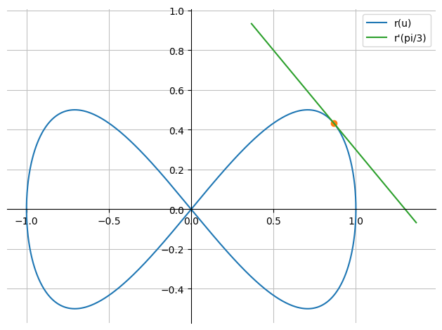
We are given a parameter curve for \(u \in [0, 2\pi]\):

u = symbols('u', real=True)
r = Matrix([sin(u), sin(u)*cos(u)])
r

\[\begin{split}\displaystyle \left[\begin{matrix}\sin{\left(u \right)}\\\sin{\left(u \right)} \cos{\left(u \right)}\end{matrix}\right]\end{split}\]

p_curve = dtuplot.plot_parametric(*r, (u,0,2*pi), use_cm=False, label="r(u)",axis_center="auto")

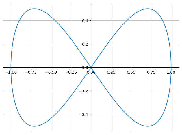
We wish to find the length of this rather unusual curve for which we have no elementary geometric formula. According to the textbook, the length can be found as a line integral if we let \(f(x)=1\).

\[\begin{equation*} L=\int_K\; \mathrm{d}\pmb{s} = \int_{0}^{2\pi} \Vert \boldsymbol r'(u) \Vert \mathrm{d}u. \end{equation*}\]

The tangent vector \(\boldsymbol r'(u)\) is:

dr = r.diff(u)
dr

\[\begin{split}\displaystyle \left[\begin{matrix}\cos{\left(u \right)}\\- \sin^{2}{\left(u \right)} + \cos^{2}{\left(u \right)}\end{matrix}\right]\end{split}\]

and it’s norm is found with a convenient command from dtutools:

Jacobian = dtutools.l2_norm(dr)

The length of the curve is thus:

L=integrate(Jacobian, (u,0,2*pi)).n()

where .n() forces the result to be shown numerically. So, the curve is around 6 units long.

Tangent Lines

Now that we have found the tangent vector, we can easily construct tangent lines from any point on the curve, should we need this, e.g. for a nice plot. Construct a tangent line as any straight line with a point on it plus a direction vector times a parameter:

\[\text{tangent line}=\boldsymbol r(u_0)+t\cdot \boldsymbol r'(u_0)\,,\quad t\in\Bbb R.\]

The tangent line at, for example, \(x_0=r(\pi/3)\) is parametrized as follows, for \(t\in \Bbb R\):

t = symbols("t")
r_tan = r.subs(u,pi/3) + t*dr.subs(u,pi/3)
r_tan

\[\begin{split}\displaystyle \left[\begin{matrix}\frac{t}{2} + \frac{\sqrt{3}}{2}\\- \frac{t}{2} + \frac{\sqrt{3}}{4}\end{matrix}\right]\end{split}\]

p_point = dtuplot.scatter(r.subs(u,pi/3), show=False)
p_tan = dtuplot.plot_parametric(*r_tan, (t,-1,1), use_cm=False, label="r'(pi/3)", show=False)

(p_curve + p_point + p_tan).show()

A Line Integral along a Space Curve

We are now given a function:

x,y,z = symbols("x y z")
f = lambda x,y,z: sqrt(x**2 + y**2 + z**2)
f(x,y,z)

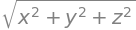
and a parameter curve \(K\) for \(u\in[0,5]\) - as we are in 3D space, this is known as a space curve:

u = symbols('u', real=True)
r = Matrix([u*cos(u), u*sin(u), u])
r

\[\begin{split}\displaystyle \left[\begin{matrix}u \cos{\left(u \right)}\\u \sin{\left(u \right)}\\u\end{matrix}\right]\end{split}\]

p_spacecurve = dtuplot.plot3d_parametric_line(*r, (u,0,2*pi), use_cm=False, label="r(u)",aspect="equal", legend=True)

Let’s compute the line integral:

\[\int_K f(x,y,z)\, \mathrm{d}\pmb{s}= \int_{0}^{5} \,f(\boldsymbol r(u))\,\Vert \boldsymbol r'(u) \Vert \mathrm{d}u.\]

The tangent vector and its norm (our Jacobian function):

dr = r.diff(u)
Jacobian = dr.norm().simplify()
Jacobian

Note: Had u not been defined as a real variable with symbols('u', real=True), then dr.norm() couldn’t be used and you would instead have to use dtutools.l2_norm(dr).

The restriction:

restriction = f(*r).simplify()
restriction

All components are ready, and we find the line integral along the curve:

integrate( restriction * Jacobian ,(u,0,5)).evalf()

Should we be in need of its length, then we simply leave out the function:

integrate(Jacobian,(u,0,5)).evalf()

Assumptions

Notice that our restriction in the above line integral calculation contains an absolute-value symbol, \(|u|\):

restriction

Often, Sympy doesn’t mind and can do an integration with it just fine, as we saw above. But should the integrations be more advanced and make Sympy struggle or spend a long time, then we can give Sympy a hand by handling this absolute value manually first.

In this case, since \(u\in [0, 5]\) then \(u\) is always positive and the absolute-value symbol can be removed without consequence. Sympy does not know that from the definition u = symbols('u', real=True), so we could redefine as

u = symbols('u', real=True, nonnegative=True)

restriction

If Sympy does not automatically reduce the absolute-value lines away, then use refine():

refine(restriction, Q.nonnegative(u))

Q.nonnegative(u) enforces the assumption of non-negativity. For other assumptions, replace the .nonnegative() part with other entries in this table.

Surface Integrals

Consider a function \(f: \mathbb{R}^3 \to \mathbb{R}\) given by

\[\begin{equation*} f(x,y,z) = 8 z. \end{equation*}\]

x,y,z = symbols('x y z', real=True)
def f(x,y,z):
    return 8*z

f(x,y,z)

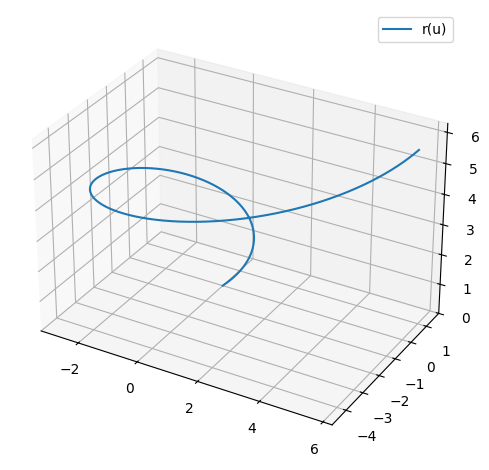
Also consider a surface \(S\) given by the following parametric representation, where \(u \in [0,\frac{\pi}{2}],v \in [0,1]\):

u,v = symbols('u v', real=True, nonnegative=True)
r = Matrix([u*cos(u),u*sin(u),u*v])
r

\[\begin{split}\displaystyle \left[\begin{matrix}u \cos{\left(u \right)}\\u \sin{\left(u \right)}\\u v\end{matrix}\right]\end{split}\]

This time we remembered nonnegative=True as, again, neither \(u\) nor \(v\) can be negative. This geometry is known as a cylinder surface since it extends upwards like a piece of a cylindrical “wall”:

dtuplot.plot3d_parametric_surface(*r,(u,0,pi/2),(v,0,1), aspect='equal')

<spb.backends.matplotlib.matplotlib.MatplotlibBackend at 0x7ff4698eb010>

Our job is to find the surface integral of \(f\) over the surface \(S\). For that we employ the change-of-variables theorem, for which the textbook gives us this formula for our case:

\[\begin{equation*} \int_S f\; \mathrm{d}\pmb{A} = \int_{0}^{1} \int_{0}^{\pi/2} f(\boldsymbol r_S(u,v))\cdot||\frac{\partial \boldsymbol r_C}{\partial u}\times \frac{\partial \boldsymbol r_C}{\partial v}||\;\mathrm{d}u\,\mathrm{d}v. \end{equation*}\]

The Jacobian function is this time the norm of the cross product between the two partial derivatives of the parametrization:

crossproduct = r.diff(u).cross(r.diff(v))
Jacobian = sqrt((crossproduct.T * crossproduct)[0]).simplify()
Jacobian

The integrand:

integrand = f(*r) * Jacobian
integrand

The surface integral:

integrate(integrand,(v,0,1),(u,0,pi/2)).evalf()

Had we preferred the area of the surface, then we would simply leave out the function, as always:

A=integrate(Jacobian,(v,0,1),(u,0,pi/2)).evalf()
A