Demo 11: Integration of Vector Fields through Surfaces (Flux)

Demo by Christian Mikkelstrup, Hans Henrik Hermansen, Jakob Lemvig, Karl Johan Måstrup Kristensen, and Magnus Troen. Revised March 2026 by shsp.

from sympy import *
from dtumathtools import *

init_printing()

Flux through a surface \(F\) is, according to the textbook, found as an orthogonal surface integral, and the formula simplifies to the following:

(5)\[\begin{equation} \int_F\boldsymbol V\cdot \mathrm d\boldsymbol S = \int_a^b\int_c^d \pmb{V}(\boldsymbol r(u,v))\cdot \boldsymbol N\,\mathrm{d}u\,\mathrm{d}v. \end{equation}\]

This uses the canonical normal vector \(\boldsymbol N\), calculated as a cross product of the partial derivatives of the surface parametrization, \(\boldsymbol N=\frac{\partial \boldsymbol r}{\partial u}\times \frac{\partial \boldsymbol r}{\partial v}\). We clearly see that the direction of this normal vector will determine the sign of the flux; i.e., vector field vectors along with \(\boldsymbol N\) give positive contributions since the dot product then is positive, and so on. Thus, the normal vector indicates our choice of positive orientation which allows us to understand the sign of the resulting flux.

Flux through Closed Paraboloid

We are given a vector field by:

x, y, z = symbols("x y z", real=True)
V = lambda x, y, z: Matrix([x, y, 2])
V(x, y, z)

\[\begin{split}\displaystyle \left[\begin{matrix}x\\y\\2\end{matrix}\right]\end{split}\]

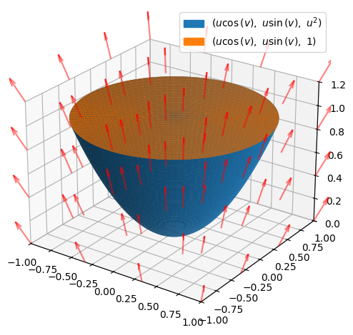
Let’s consider the paraboloidal container with a lid from demo 8, which we parametrized in two parts as:

u, v = symbols("u v", real=True)
r_wall = Matrix([u * cos(v), u * sin(v), u**2])
r_lid = Matrix([u * cos(v), u * sin(v), 1])
r_wall, r_lid

\[\begin{split}\displaystyle \left( \left[\begin{matrix}u \cos{\left(v \right)}\\u \sin{\left(v \right)}\\u^{2}\end{matrix}\right], \ \left[\begin{matrix}u \cos{\left(v \right)}\\u \sin{\left(v \right)}\\1\end{matrix}\right]\right)\end{split}\]

both defined for \(u\in [0,1],v\in [-\pi,\pi]\). The vector field and the surface in one plot:

p_wall = dtuplot.plot3d_parametric_surface(*r_wall,(u, 0, 1),(v, -pi, pi),
    use_cm=False,
    camera={"elev": 25, "azim": -55},
    show=False
)
p_lid = dtuplot.plot3d_parametric_surface(*r_lid,(u, 0, 1),(v, -pi, pi),
    show=False
)
p_field = dtuplot.plot_vector(V(x, y, z),(x, -1, 1),(y, -1, 1),(z, 0, 1.2),
    n=4,
    use_cm=False,
    quiver_kw={"alpha": 0.5, "length": 0.1, "color": "red"},
    show=False,
)

(p_wall + p_lid + p_field).show()

Normal Vector

Let’s compute the flux (the orthogonal surface integral) of the vector field out through this closed paraboloidal container. I.e., we want normal vectors that point outwards from the container from any point on both parts of the surface. The first step will therefore be to check the normal vector direction for both pieces of the surface.

Normal vector for the paraboloidal wall:

n_wall = r_wall.diff(u).cross(r_wall.diff(v))
simplify(n_wall)

\[\begin{split}\displaystyle \left[\begin{matrix}- 2 u^{2} \cos{\left(v \right)}\\- 2 u^{2} \sin{\left(v \right)}\\u\end{matrix}\right]\end{split}\]

It points inwards into the container, so let’s switch the order of the vectors:

n_wall = r_wall.diff(v).cross(r_wall.diff(u))
simplify(n_wall)

\[\begin{split}\displaystyle \left[\begin{matrix}2 u^{2} \cos{\left(v \right)}\\2 u^{2} \sin{\left(v \right)}\\- u\end{matrix}\right]\end{split}\]

Great. Alternatively, we could just change the sign of the normal vector. Or, even simpler, we could just remember that the orientation is wrong until we are done, and then simply change the sign of the flux. But here we chose the fix of switching vectors around.

Next, the normal vector for the lid:

n_lid = r_lid.diff(u).cross(r_lid.diff(v))
simplify(n_lid)

\[\begin{split}\displaystyle \left[\begin{matrix}0\\0\\u\end{matrix}\right]\end{split}\]

It points upwards, which fits with our intended outwards orientation. No change needed here.

The Flux

Let’s plot along with the paraboloidal wall only those vectors from the vector field that start from the wall. We do that with a slice argument on plot_vector:

parab_surface = dtuplot.plot3d_parametric_surface(*r_wall, (u, 0, 1), (v, -pi, pi), n=8, show=False)

p_field2 = dtuplot.plot_vector(V(x, y, z),(x, -1, 1),(y, -1, 1),(z, 0, 1),
    slice=parab_surface[0],
    use_cm=False,
    quiver_kw={"alpha": 0.5, "length": 0.1, "color": "red"},
    show=False,
)
p_wall.camera = {"elev": 60, "azim": -50}

(p_wall + p_field2).show()

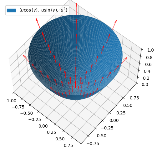
Notice that vectors arrive from all corners. There are too many vectors when p_wall is shown along with them, so here we reduce n a bit to show fewer arrows. The plot seems to show that the flow is upwards throught the container. With outwards-pointing normal vectors, we would thus expect a net negative flux through the paraboloidal wall and a net positive flux through the lid.

Their sum is the total flux through the container. Let’s find them individually - first for the paraboloidal wall:

integrand_wall = n_wall.dot(V(*r_wall))
Flux_wall = integrate(integrand_wall, (u, 0, 1), (v, -pi, pi))
Flux_wall

The flux out through the paraboloidal wall is \(-\pi\). It is negative as suspected.

Now, the lid:

integrand_lid = n_lid.dot(V(*r_lid))
Flux_lid = integrate(integrand_lid, (u, 0, 1), (v, -pi, pi))
Flux_lid

The flux through the lid is \(2\pi\), positive as suspected. The total flux:

Flux = Flux_lid + Flux_wall

The total flux through the closed container as a whole is thus \(\mathrm{Flux}(\pmb{V},F_{wall}\cup F_{lid})=-\pi+2\pi=\pi\). The total flux is positive, so there is a net outwards flow from inside the container.

Flux through Segment of Spherical Shell

We are given a vector field,

x, y, z = symbols("x y z")
V = Matrix([-y + x, x, z])
V

\[\begin{split}\displaystyle \left[\begin{matrix}x - y\\x\\z\end{matrix}\right]\end{split}\]

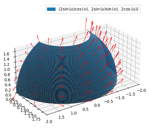
and a section of a spherical surface,

u, v, w = symbols("u v w", real=True)
radius = 2
r = radius * Matrix([sin(u) * cos(v), sin(u) * sin(v), cos(u)])
r

\[\begin{split}\displaystyle \left[\begin{matrix}2 \sin{\left(u \right)} \cos{\left(v \right)}\\2 \sin{\left(u \right)} \sin{\left(v \right)}\\2 \cos{\left(u \right)}\end{matrix}\right]\end{split}\]

where \(u\in[\pi/6,\pi/2],v\in[0,\pi]\).

p_surface = dtuplot.plot3d_spherical(
    radius,
    (u, pi / 6, pi / 2),(v, 0, pi),
    aspect="equal",
    camera={"elev": 25, "azim": 55},
    show=False,
)
dummy_surface = dtuplot.plot3d_spherical(
    radius, (u, pi / 6, pi / 2), (v, 0, pi), show=False, n=8
)
p_field = dtuplot.plot_vector(
    V,
    (x, -1, 1),(y, -1, 1),(z, 0, 1),
    slice=dummy_surface[0],
    use_cm=False,
    quiver_kw={"alpha": 0.5, "length": 0.2, "color": "red"},
    show=False,
)

(p_surface + p_field).show()

The normal vector:

n = r.diff(u).cross(r.diff(v))
n

\[\begin{split}\displaystyle \left[\begin{matrix}4 \sin^{2}{\left(u \right)} \cos{\left(v \right)}\\4 \sin^{2}{\left(u \right)} \sin{\left(v \right)}\\4 \sin{\left(u \right)} \sin^{2}{\left(v \right)} \cos{\left(u \right)} + 4 \sin{\left(u \right)} \cos{\left(u \right)} \cos^{2}{\left(v \right)}\end{matrix}\right]\end{split}\]

As we have no desired orientation, no adjustment is needed. But we still need to know the direction of the normal vector to interpret the flux correctly. This normal vector points away from the centre of the sphere segment.

The flux is computed to be

integrand = n.dot(V.subs({x: r[0], y: r[1], z: r[2]}))
integrate(integrand, (u, pi / 6, pi / 2), (v, 0, pi))

A positive value, so the net flow is along the normal vector, that is, outwards/away from the sphere centre.

Flux through Solid Semi-Sphere

Consider in \(\Bbb R^3\) a solid semi-sphere with radius \(a\) parametrized as follows, for \(u\in[0,a]\), \(v\in[0,\pi/2]\), and \(w\in[-\pi,\pi]\), as well as a vector field \(\boldsymbol V\):

x,y,z,u,v,w=symbols('x y z u v w')
a = symbols("a", real=True, positive=True)
V = Matrix([8 * x, 8, 4 * z**3])
r = u * Matrix([sin(v) * cos(w), sin(v) * sin(w), cos(v)])
V, r

\[\begin{split}\displaystyle \left( \left[\begin{matrix}8 x\\8\\4 z^{3}\end{matrix}\right], \ \left[\begin{matrix}u \sin{\left(v \right)} \cos{\left(w \right)}\\u \sin{\left(v \right)} \sin{\left(w \right)}\\u \cos{\left(v \right)}\end{matrix}\right]\right)\end{split}\]

We wish to compute the flux through the closed boundary surface of this solid object. The surface consists of two pieces that we’ll handle individually. The first surface segment is obtained by fixing \(u\) to the radius value \(a\):

r1 = r.subs(u, a)
n1 = r1.diff(v).cross(r1.diff(w))
integrand1 = n1.dot(V.subs({x: r1[0], y: r1[1], z: r1[2]}))
flux1 = integrate(integrand1, (v, 0, pi / 2), (w, -pi, pi))
r1,n1,flux1

\[\begin{split}\displaystyle \left( \left[\begin{matrix}a \sin{\left(v \right)} \cos{\left(w \right)}\\a \sin{\left(v \right)} \sin{\left(w \right)}\\a \cos{\left(v \right)}\end{matrix}\right], \ \left[\begin{matrix}a^{2} \sin^{2}{\left(v \right)} \cos{\left(w \right)}\\a^{2} \sin^{2}{\left(v \right)} \sin{\left(w \right)}\\a^{2} \sin{\left(v \right)} \sin^{2}{\left(w \right)} \cos{\left(v \right)} + a^{2} \sin{\left(v \right)} \cos{\left(v \right)} \cos^{2}{\left(w \right)}\end{matrix}\right], \ \frac{8 \pi a^{5}}{5} + \frac{16 \pi a^{3}}{3}\right)\end{split}\]

The second surface segment corresponds to fixing \(v\) to the value \(\pi/2\), which becomes a disc with radius \(a\):

r2 = r.subs(v, pi / 2)
n2 = r2.diff(u).cross(r2.diff(w))
integrand2 = n2.dot(V.subs({x: r2[0], y: r2[1], z: r2[2]}))
flux2 = integrate(integrand2, (u, 0, a), (w, -pi, pi))
r2,n2,flux2

\[\begin{split}\displaystyle \left( \left[\begin{matrix}u \cos{\left(w \right)}\\u \sin{\left(w \right)}\\0\end{matrix}\right], \ \left[\begin{matrix}0\\0\\u \sin^{2}{\left(w \right)} + u \cos^{2}{\left(w \right)}\end{matrix}\right], \ 0\right)\end{split}\]

Can we now simply add the two fluxes together to obtain the total flux through this solid semi-sphere? Be careful! We must first check that their normal vectors are in agreement - otherwise the signs of the two fluxes won’t match.

After checking we see that the normal vectors of the first surface segment point outwards, but those of the second segment point inwards. So, the signs of the fluxes do not match. To fix this, let’s change the sign of the flux through the second segment:

flux_through_semisphere = flux1 + (-flux2)
flux_through_semisphere

This result should now be understood with an outwards positive orientation. Note that whether the normal vectors point outwards or inwards is not important, as long as they are in agreement!

Gauss’ Divergence Theorem (Not Syllabus)

The rest of this demo contains material that might be relevant for some students for the project period in Mathematics 1b, but that is not a part of the course curriculum.

Gauss’ Theorem is a very useful theorem in the context of flux computations through closed surfaces. It let’s you find the flux through a closed surface by “pushing the computation to the interior” in case that is easier. More specifically, if we consider the closed surface as the boundary of a solid region \(\Omega\), then Gauss’ Theorem states that the flux out through this surface \(\partial \Omega\) is equal to the volume integral of the divergence of the vector field through \(\Omega\):

\[\mathrm{Flux}(\boldsymbol V,\partial \Omega)=\int_{\partial \Omega}\boldsymbol V\cdot \mathrm d\boldsymbol S=\int_{\Omega}\mathrm{div}(\boldsymbol V) \mathrm dS.\]

Flux through Solid Semi-Sphere with Gauss’ Theorem (Not Syllabus)

Consider once again the vector field \(\boldsymbol V\) and solid semi-sphere parametrized by \(\boldsymbol r\) that we calculated the flux through in the previous section:

V, r

\[\begin{split}\displaystyle \left( \left[\begin{matrix}8 x\\8\\4 z^{3}\end{matrix}\right], \ \left[\begin{matrix}u \sin{\left(v \right)} \cos{\left(w \right)}\\u \sin{\left(v \right)} \sin{\left(w \right)}\\u \cos{\left(v \right)}\end{matrix}\right]\right)\end{split}\]

Here \(u\in[0,a],v\in[0,\pi/2],w\in[-\pi,\pi]\). We found the flux to be:

flux_through_semisphere

As this is a closed surface, Gauss’ Theorem will apply. Let’s see if we can get the same result using Gauss’ Theorem. For that we will be doing a volume integral of the divergence of the vector field through the semi-sphere’s interior.

For the volume integral, we need the determinant of the Jacobian matrix:

M = Matrix.hstack(r.diff(u), r.diff(v), r.diff(w))
jacobian = M.det()
jacobian

We should also take the absolute value of it, but the determinant is always positive, since the only term that is not squared is \(\sin(v)\), which is positive within \(v\)’s interval. Next, the divergence of the vector field:

divV = dtutools.div(V, [x, y, z])
divV_r = divV.subs({x: r[0], y: r[1], z: r[2]})
divV,divV_r

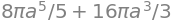
and we have right away restricted \(\mathrm{div}\boldsymbol V\) to the parametrization as well. Finally, the volume integration, which here is a triple integral:

integrate(divV_r * jacobian, (u, 0, a), (v, 0, pi / 2), (w, -pi, pi))

The result is the same, as expected!

Note that we have not considered orientation here. The reason is that Gauss’ Theorem automatically assumes an outwards positive orientation. That the result matches what we found earlier is because we ended up choosing an outwards orientation in the previous flux calculation.

Flux through a Ramp (Not Syllabus)

We are given the vector field

V = Matrix([-x + cos(z), -y * x, 3 * z + exp(y)])
V

\[\begin{split}\displaystyle \left[\begin{matrix}- x + \cos{\left(z \right)}\\- x y\\3 z + e^{y}\end{matrix}\right]\end{split}\]

and we consider the spatial region \(\Omega\) that we parametrized in demo 8 as follows for \(u\in[0,3],v\in[0,2],w\in[0,1]\):

u, v, w = symbols("u v w")
r = Matrix([u, v, w * v**2])
r

\[\begin{split}\displaystyle \left[\begin{matrix}u\\v\\v^{2} w\end{matrix}\right]\end{split}\]

a = symbols("a")
p = dtuplot.plot3d_parametric_surface(
    x,
    y,
    y**2,
    (x, 0, 3),
    (y, 0, 2),
    {"color": "royalblue"},
    use_cm=False,
    aspect="equal",
    show=False,
)
p.extend(
    dtuplot.plot3d_parametric_surface(
        0,
        y,
        a * y**2,
        (a, 0, 1),
        (y, 0, 2),
        {"color": "royalblue", "alpha": 0.5},
        use_cm=False,
        aspect="equal",
        show=False,
    )
)
p.extend(
    dtuplot.plot3d_parametric_surface(
        3,
        y,
        a * y**2,
        (a, 0, 1),
        (y, 0, 2),
        {"color": "royalblue", "alpha": 0.5},
        use_cm=False,
        aspect="equal",
        show=False,
    )
)
p.extend(
    dtuplot.plot3d_parametric_surface(
        x,
        2,
        a * 4,
        (x, 0, 3),
        (a, 0, 1),
        {"color": "royalblue", "alpha": 0.5},
        use_cm=False,
        aspect="equal",
        show=False,
    )
)
p.extend(
    dtuplot.plot3d_parametric_surface(
        x,
        y,
        0,
        (x, 0, 3),
        (y, 0, 2),
        {"color": "royalblue", "alpha": 0.5},
        use_cm=False,
        aspect="equal",
        show=False,
    )
)
p_field = dtuplot.plot_vector(
    V,
    (x, 0, 3),
    (y, 0, 2),
    (z, 0, 4),
    n=4,
    use_cm=False,
    quiver_kw={"alpha": 0.5, "length": 0.05, "color": "red"},
    show=False,
)

(p + p_field).show()

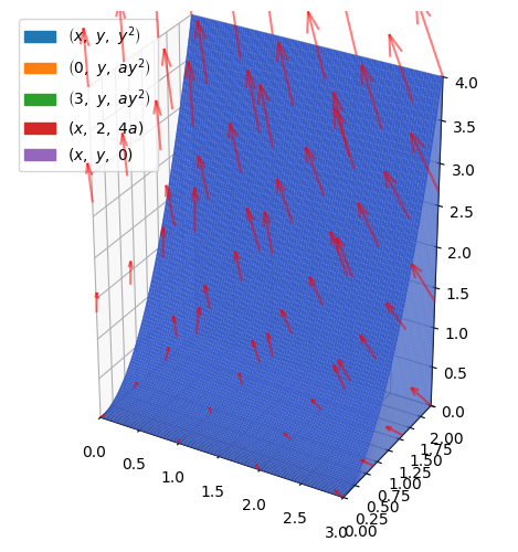
We now want to find the flux of the vector field \(\pmb{V}\) out through the boundary surface of the ramp \(\Omega\). The boundary surface of the ramp consists of many smaller segments, though, making a flux calculation with the usual flux formula rather tedious and time consuming. But Gauss’ Theorem applies for a closed surface! And this is much easier to do in this case. So, we will instead find the volume integral of the divergence of the vector field through the interior of the ramp.

The Jacobian matrix and its determinant:

M = Matrix.hstack(r.diff(u), r.diff(v), r.diff(w))
M, det(M)

\[\begin{split}\displaystyle \left( \left[\begin{matrix}1 & 0 & 0\\0 & 1 & 0\\0 & 2 v w & v^{2}\end{matrix}\right], \ v^{2}\right)\end{split}\]

We notice that \(v>0\), which makes the determinant always positive, so the Jacobian function is:

jacobian = M.det()
jacobian

The divergence:

divV = dtutools.div(V, (x, y, z))
divV

The divergence restricted to the parametrized region:

divV_r = divV.subs({x: r[0], y: r[1], z: r[2]})
divV_r

The volume integral:

integrate(divV_r * jacobian, (u, 0, 3), (v, 0, 2), (w, 0, 1))

Now, Gauss’ Theorem tells that this result is equal to the flux:

(6)\[\begin{equation} \int_{\delta\Omega}\pmb{V}\cdot \mathrm{d}\pmb{S} = \int_0^1\int_0^2\int_0^3(2-u)\cdot v^2\,\mathrm{d}u\,\mathrm{d}v\,\mathrm{d}w = 4. \end{equation}\]

This example makes it clear that Gauss’ Theorem can save us a lot of work: We avoided having to compute the fluxes through five surfaces, requiring five parametrizations with five Jacobians, that then would be added to the total flux. Instead we had to just do one parametrization and find its one Jacobian. Sure, we do have to compute with one more integration and we also have to first find the divergence. Whether Gauss’ Theorem will save you time or whether you’ll want to stick with the usual approach to calculating flux, depends entirely on the situation.