Demo 10: Vector Fields and their Integration along Curves (the Tangential Line Integral)

Demo by Christian Mikkelstrup, Hans Henrik Hermansen, Jakob Lemvig, Karl Johan Måstrup Kristensen, and Magnus Troen. Revised March 2026 by shsp.

from sympy import *
from dtumathtools import *

init_printing()

Vector Fields

Vector fields can be defined, as any other vector functions, either as a Sympy expression,

x, y, z = symbols("x,y,z", real=True)

V = Matrix([y * cos(x), y * sin(x), z])
V

\[\begin{split}\displaystyle \left[\begin{matrix}y \cos{\left(x \right)}\\y \sin{\left(x \right)}\\z\end{matrix}\right]\end{split}\]

or as a Python function, e.g., as a lambda function:

V = lambda x, y, z: Matrix([y * cos(x), y * sin(x), z])
V(x, y, z)

\[\begin{split}\displaystyle \left[\begin{matrix}y \cos{\left(x \right)}\\y \sin{\left(x \right)}\\z\end{matrix}\right]\end{split}\]

You will often need to substitute parametric representations, which are vector functions themselves, into vector fields, and for that the latter definition above is more convenient. A parameter curve,

\[\begin{equation*} \boldsymbol{r} = \begin{bmatrix} r_1(t) \\ r_2(t) \\ r_3(t) \end{bmatrix}, \end{equation*}\]

r1, r2, r3 = symbols("r1,r2,r3", cls=Function)
t = symbols("t")
r = Matrix([r1(t), r2(t), r3(t)])

is easily substituted into the vector field with:

V(*r)

\[\begin{split}\displaystyle \left[\begin{matrix}r_{2}{\left(t \right)} \cos{\left(r_{1}{\left(t \right)} \right)}\\r_{2}{\left(t \right)} \sin{\left(r_{1}{\left(t \right)} \right)}\\r_{3}{\left(t \right)}\end{matrix}\right]\end{split}\]

On the other hand, having to type out V(x,y,z) every time you use the vector field can be cumbersome, in which case the former definition lets you type just V.

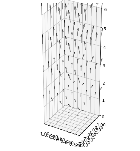
Plotting of vector fields is easy. Note the styling of the arrows:

vectorfield_V = dtuplot.plot_vector(
    V(x,y,z),
    (x, -1, 1),(y, -1, 1),(z, 0, 6),
    n=5,
    quiver_kw={"alpha": 0.5, "length": 0.1, "color": "black"},
    colorbar=False
)

Should you ever be in need of computing more properties of a vector field, such as curl (“rotation”) or divergence, then you’ll find commands for it in the dtumathtools package:

rotV = dtutools.rot(V(x, y, z), (x, y, z))
rotV

\[\begin{split}\displaystyle \left[\begin{matrix}0\\0\\y \cos{\left(x \right)} - \cos{\left(x \right)}\end{matrix}\right]\end{split}\]

divV = dtutools.div(V(x, y, z), (x, y, z))
divV

The Tangential Line Integral

Consider the vector field

\[\begin{equation*} \pmb{V}(x,y,z) = \begin{bmatrix} -y \\ x \\ 2z \end{bmatrix} \end{equation*}\]

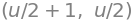
along with two curves \(K_1\) and \(K_2\) with the parametric representations

\[\begin{equation*} \boldsymbol r_1(u) = \begin{bmatrix} \cos(u) \\ \sin(u) \\ \frac{u}{2} \end{bmatrix}\,, \qquad \boldsymbol r_2(u) = \begin{bmatrix} 1 \\ 0 \\ \frac{u}{2} \end{bmatrix}, \end{equation*}\]

respectively, where \(u \in [0,4\pi]\) for both.

x, y, z, u = symbols("x y z u", real=True)
r1 = Matrix([cos(u), sin(u), u / 2])
r2 = Matrix([1, 0, u / 2])
V = Matrix([-y, x, 2 * z])
u_range = (u, 0, 4 * pi)

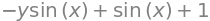
Geometrically, \(\boldsymbol r_1\) draws a segment of a helix while \(\boldsymbol r_2(u)\) draws a vertical line segment. Note that they both start at \(A = (1,0,0)\) and end at \(B = (1,0,2\pi)\). Let’s view a combined plot:

K1 = dtuplot.plot3d_parametric_line(
    *r1, u_range, show=False, rendering_kw={"color": "red"}, colorbar=False
)
K2 = dtuplot.plot3d_parametric_line(
    *r2, u_range, show=False, rendering_kw={"color": "blue"}, colorbar=False
)
vectorfield_V = dtuplot.plot_vector(V,(x, -1, 1),(y, -1, 1),(z, 0, 6),
    n=5,
    quiver_kw={"alpha": 0.5, "length": 0.1, "color": "black"},
    colorbar=False,
    show=False,
)

combined = K1 + K2 + vectorfield_V
combined.legend = False
combined.show()

We wish to compute the tangential line integral of \(\pmb{V}\) along each of the two curves from \(A\) to \(B\). The textbook gives us the formula (where \(a\) and \(b\) are the \(u\) values that represent the points \(A\) and \(B\), respectively, meaning \(A=\boldsymbol r(a),B=\boldsymbol r(b)\)):

\[\begin{equation*} \int_{K} \pmb{V} \cdot \mathrm{d}\pmb{s} = \int_a^b \pmb{V}(\boldsymbol r(u))\cdot \boldsymbol r'(u) \,\mathrm{d}u. \end{equation*}\]

First, their tangent vectors:

r1d = r1.diff(u)
r2d = r2.diff(u)
r1d, r2d

\[\begin{split}\displaystyle \left( \left[\begin{matrix}- \sin{\left(u \right)}\\\cos{\left(u \right)}\\\frac{1}{2}\end{matrix}\right], \ \left[\begin{matrix}0\\0\\\frac{1}{2}\end{matrix}\right]\right)\end{split}\]

Then the integrands, which are dot products:

integrand1 = V.subs({x: r1[0], y: r1[1], z: r1[2]}).dot(r1d)
integrand2 = V.subs({x: r2[0], y: r2[1], z: r2[2]}).dot(r2d)
integrand1.simplify(), integrand2.simplify()

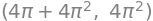
So, the tangential line integral along \(K_1\) is found as \(\int_{K_1} \pmb{V} \cdot \mathrm{d}\pmb{s} = \int_0^{4\pi} \frac{u}{2} + 1 \,\mathrm{d}u\) and along \(K_2\) as \(\int_{K_2} \pmb{V} \cdot \mathrm{d}\pmb{s} = \int_0^{4\pi} \frac{u}{2} \,\mathrm{d}u\):

Tan_K1=integrate(integrand1, (u, 0, 4 * pi))
Tan_K2=integrate(integrand2, (u, 0, 4 * pi))
Tan_K1,Tan_K2

They are not equal, which means that the tangential line integral is path-dependent. In the textbook we see the consequences of this, for instance that \(\boldsymbol V\) cannot be a gradient vector field (i.e., it has no antiderivative).

In a physical interpretation, if \(\pmb{V}\) is a force field, then it will do work on a particle that moves through it. The tangential line integral is this amount of total work. When moving along the vertical line, the work done on the particle is apparently less than when moving along the helix. The amounts are both positive, so in both cases the force field helps the particle along from \(A\) to \(B\) by pushing it forwards overall, and it helps out more (more kinetic energy will have been added by the force field) when following the helix. Should the particle move from \(B\) to \(A\), though, then the magnitudes will be the same but the signs will be opposite, since we are flipping the integration limits.

Gradient Vector Fields and Anti-Derivatives

According to the textbook, if a smooth vector field is a gradient vector field, then:

• it has an antiderivative (that is, a function of which it is the gradient).

• a tangential line integral of it along any curve from the origin to an arbitrary point \(\pmb{x}\) will be an antiderivative.

• tangential line integrals of it are path-independent.

Knowing that a vector field is a gradient vector field is thus very useful. We can check for that by computing the tangential line integral along any path after which we can check whether the first bullet point is fulfilled. As we can choose any path, an often-used choice is a so-called stair line.

The Stair-Line Method

Let’s consider a smooth vector field in \(\Bbb R^3\):

\[\begin{equation*} \pmb{V}(x,y,z) = \begin{bmatrix} V_1(x,y,z) \\ V_2(x,y,z) \\ V_3(x,y,z) \end{bmatrix}. \end{equation*}\]

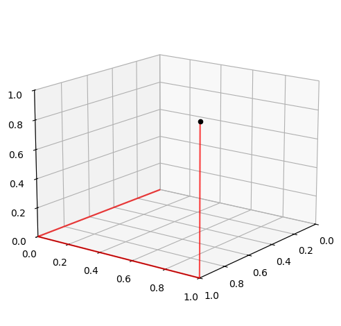
By the stair line \(T\) from the origin \(\pmb{x}_0=(0,0,0)\) to an arbitrary point \(\pmb{x}=(x,y,z)\) we mean the path you would follow if you had to walk along the \(x\) axis, then along the \(y\) axis, and then along the \(z\) axis. These three segments are axis-parallel straight lines and thus easy to parametrize:

\[\begin{split}\boldsymbol r_1(u)=(u,0,0)\,,\,u\in[0,x]\\ \boldsymbol r_2(u)=(x,u,0)\,,\,u\in[0,y]\\ \boldsymbol r_3(u)=(x,y,u)\,,\,u\in[0,z].\end{split}\]

r1 = Matrix([u, 0, 0])
r2 = Matrix([x, u, 0])
r3 = Matrix([x, y, u])

For \((x,y,z)=(1,1,1)\) as an example point, a plot of the stair line becomes:

u_range = (u, 0, 1)

# The stair line steps
p1 = dtuplot.plot3d_parametric_line(u, 0, 0, u_range, show=False, rendering_kw={"color": "red"}, colorbar=False)
p2 = dtuplot.plot3d_parametric_line(1, u, 0, u_range, show=False, rendering_kw={"color": "red"}, colorbar=False)
p3 = dtuplot.plot3d_parametric_line(1, 1, u, u_range, show=False, rendering_kw={"color": "red"}, colorbar=False)

# The point
xyz = dtuplot.scatter(Matrix([1, 1, 1]), show=False, rendering_kw={"color": "black"})

combined = p1 + p2 + p3 + xyz
combined.legend = False
combined.camera = {"azim": 37, "elev": 16}

combined.show()

A tangential line integral of \(\boldsymbol V\) along the stair line \(T\) can be found as the sum of the tangential line integrals along each of the three line segments. And here we see the advantage of the stair-line method, because their three tangent vectors are very simple:

r1d = r1.diff(u)
r2d = r2.diff(u)
r3d = r3.diff(u)
r1d, r2d, r3d

\[\begin{split}\displaystyle \left( \left[\begin{matrix}1\\0\\0\end{matrix}\right], \ \left[\begin{matrix}0\\1\\0\end{matrix}\right], \ \left[\begin{matrix}0\\0\\1\end{matrix}\right]\right)\end{split}\]

which makes their three integrands particularly simple as well:

\[\begin{equation*} \begin{aligned} \pmb{V}(\boldsymbol r_1(u)) \cdot \boldsymbol r_1'(u) = V_1(u,0,0),\\ \pmb{V}(\boldsymbol r_2(u)) \cdot \boldsymbol r_2'(u) = V_2(x,u,0),\\ \pmb{V}(\boldsymbol r_3(u)) \cdot \boldsymbol r_3'(u) = V_3(x,y,u). \end{aligned} \end{equation*}\]

Hence, we have the following simple formula for the tangential line integral of \(\pmb{V}\) along a stair line to an arbitrary point in \(\Bbb R^3\):

\[\begin{equation*} \int_T \pmb{V} \cdot \mathrm{d}\pmb{s} = \int_0^x V_1(u,0,0) \,\mathrm{d}u + \int_0^y V_2(x,u,0) \,\mathrm{d}u +\int_0^z V_3(x,y,u) \,\mathrm{d}u. \end{equation*}\]

Gradient Field or Not?

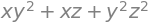
We wish to investigate whether the following vector field \(\pmb{V}\) is a gradient vector field:

\[\begin{equation*} \pmb{V}(x,y,z) = \begin{bmatrix} y^2 + z \\ 2yz^2 + 2yx \\ 2y^2z + x \end{bmatrix}. \end{equation*}\]

V = Matrix([y**2 + z, 2 * y * z**2 + 2 * y * x, 2 * y**2 * z + x])
V

\[\begin{split}\displaystyle \left[\begin{matrix}y^{2} + z\\2 x y + 2 y z^{2}\\x + 2 y^{2} z\end{matrix}\right]\end{split}\]

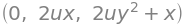
Let’s find the tangential line integral of \(\pmb{V}\) along a stair line to an arbitrary point. Using the formula we found in the previous subsection that splits the integration into three, the corresponding three integrands become:

integrand1 = V[0].subs({x: u, y: 0, z: 0})
integrand2 = V[1].subs({y: u, z: 0})
integrand3 = V[2].subs({z: u})

integrand1, integrand2, integrand3

The tangential line integral is then:

F = (integrate(integrand1,(u,0,x)) + integrate(integrand2,(u,0,y)) + integrate(integrand3,(u,0,z)))
F

This is a function in \(x,y,z\). Let’s find its gradient:

F_grad = dtutools.gradient(F)
F_grad, Eq(F_grad, V)

\[\begin{split}\displaystyle \left( \left[\begin{matrix}y^{2} + z\\2 x y + 2 y z^{2}\\x + 2 y^{2} z\end{matrix}\right], \ \text{True}\right)\end{split}\]

As \(\pmb{V}\) is identical to the gradient of \(F\), then \(F\) is an anti-derivative to \(\pmb{V}\) and \(\pmb{V}\) is a gradient vector field!

Circulation in a Gradient Vector Field

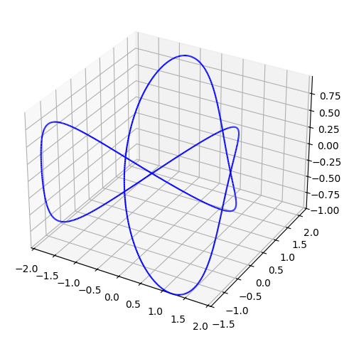
Consider the vector field \(\pmb{V}\) from the previous subsection as well as the following knot, parametrized with \(t \in[-\pi,\pi]\):

t = symbols("t")
knot = (
    Matrix([-10 * cos(t) - 2 * cos(5 * t) + 15 * sin(2 * t),
            -15 * cos(2 * t) + 10 * sin(t) - 2 * sin(5 * t),
            10 * cos(3 * t)])
    *S(1)/10
)
knot

\[\begin{split}\displaystyle \left[\begin{matrix}\frac{3 \sin{\left(2 t \right)}}{2} - \cos{\left(t \right)} - \frac{\cos{\left(5 t \right)}}{5}\\\sin{\left(t \right)} - \frac{\sin{\left(5 t \right)}}{5} - \frac{3 \cos{\left(2 t \right)}}{2}\\\cos{\left(3 t \right)}\end{matrix}\right]\end{split}\]

dtuplot.plot3d_parametric_line(*knot, (t, -pi, pi), rendering_kw={"color": "blue"}, legend=False,colorbar=False)

<spb.backends.matplotlib.matplotlib.MatplotlibBackend at 0x7f66f9fa7f10>

A knot is a closed curve. Tangential line integrals along closed curves are also known as circulations. Let’s calculate the tangential line integral of \(\pmb{V}\) along this knot. Uncomment the following code line and run it when you are ready - but be patient as this integral may take more than a minute for Sympy to compute:

#integrate(V.subs({x: knot[0], y: knot[1], z: knot[2]}).dot(knot.diff(t)), (t, -pi, pi))

You should find the result to be \(0\).

The tangential line integral of a gradient field is path-independent and depends only on the end points, \(\boldsymbol a\) and \(\boldsymbol b\). The fundamental theorem of calculus even tells that:

\[\int_K \pmb{V} \cdot \mathrm{d}\pmb{s}=F(\boldsymbol b)-F(\boldsymbol a),\]

where \(F\) is an antiderivative. It is clear that for any closed curve within a gradient vector field, the tangential line integral will always be zero. In other words, any circulation of a gradient vector field is zero.

Integral Curves (Flow Curves)

Imagine that, at time \(t=0\), you release a particle into a force vector field at the point \(\pmb{x}_0\). How will this particle move? What trajectory will it follow? The trajectory will be a curve, whose parametrization we will denote by \(\pmb{r}(t)\), and it could be a function of time in this physical scenario. A more intuitive picture is a dust particle flowing about in the wind.

Such curves are called integral curves or sometimes flow curves. Note that it is important in the above physical analogies that the particle is considered mass-less so that inertial effects play no role - a flow curve is the path a particle will follow if it is influenced by the vector field only.

The textbook tells that flow curves are the solutions to the differential equation system:

\[\begin{equation*} \pmb{r}'(t) = \pmb V(\pmb{r}(t)), \quad \pmb{r}(0) = \pmb{x}_0, \end{equation*}\]

where \(\pmb{x}_0\) is the starting point.

Consider the vector field in \(\Bbb R^2\):

\[\begin{equation*} \pmb{V}(x,y) = \left[\begin{matrix}-\frac{1}{4}x + \frac{1}{2}y\\\frac{1}{2}x + \frac{1}{4}y\end{matrix}\right]. \end{equation*}\]

x,y = symbols('x y')
V = Matrix([-S(1)/4*x + S(1)/2*y,S(1)/2*x + S(1)/4*y])
V

\[\begin{split}\displaystyle \left[\begin{matrix}- \frac{x}{4} + \frac{y}{2}\\\frac{x}{2} + \frac{y}{4}\end{matrix}\right]\end{split}\]

Let two particles \(A\) and \(B\) start at the points \(\boldsymsol s_A\) and \(\boldsymsol s_B\), respectively:

\[\begin{equation*} s_A = (5, 0),\quad s_B = (-3, \frac{1}{2}). \end{equation*}\]

sA, sB = Matrix([5, 0]), Matrix([-3, S(1)/2])

The differential equation system that we are solving is thus:

\[\begin{equation*} \begin{bmatrix}r_1'(t)\\r_2'(t)\end{bmatrix} = \begin{bmatrix}-\frac{1}{4}r_1(t) + \frac{1}{2}r_2(t)\\\frac{1}{2}r_1(t) + \frac{1}{4}r_2(t) \end{bmatrix} =\begin{bmatrix}-\frac{1}{4} & \frac{1}{2}\\\frac{1}{2} & \frac{1}{4}\end{bmatrix} \begin{bmatrix}r_1(t)\\r_2(t)\end{bmatrix}. \end{equation*}\]

where \(\boldsymbol r = (r_1,r_2)\). Applying the initial-value condition \(\boldsymbol r(0)=\boldsymsol s_A=(5,0)\) will produce the parametrized flow curve for particle \(A\), while \(\boldsymbol r(0)=\boldsymsol s_B=(-3,\frac12)\) will produce the one for \(B\).

Note that the following approach to solving systems of ordinary differential equations (ODEs) with Sympy was covered in a Python demo in Mathematics 1a. If you need more details, we refer you to that demo.

We define the system’s matrix:

A = Matrix(2, 2, [S("-1/4"), S("1/2"), S("1/2"), S("1/4")])

and set up the unknown coordinate functions as Sympy functions and differentiate them so that we can form the above matrix equation:

r1 = Function('r1')
r2 = Function('r2')
r = Matrix([r1(t),r2(t)])

dr = diff(r,t)

ode_sys = dr - A * r
ode_sys

\[\begin{split}\displaystyle \left[\begin{matrix}\frac{r_{1}{\left(t \right)}}{4} - \frac{r_{2}{\left(t \right)}}{2} + \frac{d}{d t} r_{1}{\left(t \right)}\\- \frac{r_{1}{\left(t \right)}}{2} - \frac{r_{2}{\left(t \right)}}{4} + \frac{d}{d t} r_{2}{\left(t \right)}\end{matrix}\right]\end{split}\]

We solve it with the dsolve command from dtutools (note that everything was moved to the left-hand side in ode_sys = dr - A * r because dsolve assumes a right-hand side of zero):

dtutools.dsolve(ode_sys)

This expression describes the two coordinate functions of every flow curve. Choosing specific values for the unknown constants will settle us at a specific curve. This will be done by applying the given initial-value conditions with the ics argument:

rA_sol = dtutools.dsolve(ode_sys, ics = {r1(0):sA[0], r2(0):sA[1]})
rA_sol

rB_sol = dtutools.dsolve(ode_sys, ics = {r1(0):sB[0], r2(0):sB[1]})
rB_sol

Extracting the parametric curves:

rA = Matrix([rA_sol[r1(t)], rA_sol[r2(t)]])
rB = Matrix([rB_sol[r1(t)], rB_sol[r2(t)]])
rA, rB

\[\begin{split}\displaystyle \left( \left[\begin{matrix}\frac{\left(5 - \sqrt{5}\right) e^{\frac{\sqrt{5} t}{4}}}{2} + \frac{\left(\sqrt{5} + 5\right) e^{- \frac{\sqrt{5} t}{4}}}{2}\\\sqrt{5} e^{\frac{\sqrt{5} t}{4}} - \sqrt{5} e^{- \frac{\sqrt{5} t}{4}}\end{matrix}\right], \ \left[\begin{matrix}- \frac{\left(15 - 4 \sqrt{5}\right) e^{\frac{\sqrt{5} t}{4}}}{10} - \frac{\left(4 \sqrt{5} + 15\right) e^{- \frac{\sqrt{5} t}{4}}}{10}\\\frac{\left(5 - 11 \sqrt{5}\right) e^{\frac{\sqrt{5} t}{4}}}{20} + \frac{\left(5 + 11 \sqrt{5}\right) e^{- \frac{\sqrt{5} t}{4}}}{20}\end{matrix}\right]\right)\end{split}\]

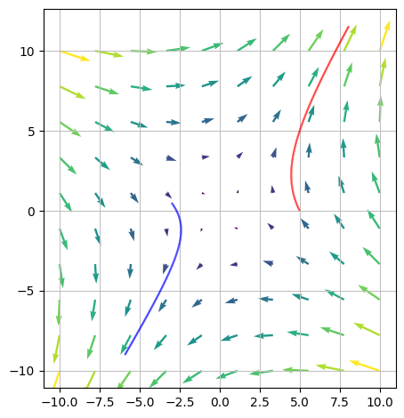
A plot of the two curves

v_field = dtuplot.plot_vector(A * Matrix([x, y]),n=10,scalar=False,colorbar=False,quiver_kw={"color": "black"},show=False)

rA_plot = dtuplot.plot_parametric(
    *rA, [t, 0, 3], rendering_kw={"color": "red"}, colorbar=False, show=False
)
rB_plot = dtuplot.plot_parametric(
    *rB, (t, 0, 4), rendering_kw={"color": "blue"}, colorbar=False, show=False
)

(v_field + rA_plot + rB_plot).show()

No ranges were provided. This function will attempt to find them, however the order will be arbitrary, which means the visualization might be flipped.